Long-Run Macroeconomic Equilibrium
Figure 12-14 combines the aggregate demand curve with both the short-run and long-run aggregate supply curves. The aggregate demand curve, AD, crosses the short-run aggregate supply curve, SRAS, at ELR. Here we assume that enough time has elapsed that the economy is also on the long-run aggregate supply curve, LRAS. As a result, ELR is at the intersection of all three curves—SRAS, LRAS, and AD. So short-run equilibrium aggregate output is equal to potential output, YP. Such a situation, in which the point of short-run macroeconomic equilibrium is on the long-run aggregate supply curve, is known as long-run macroeconomic equilibrium.
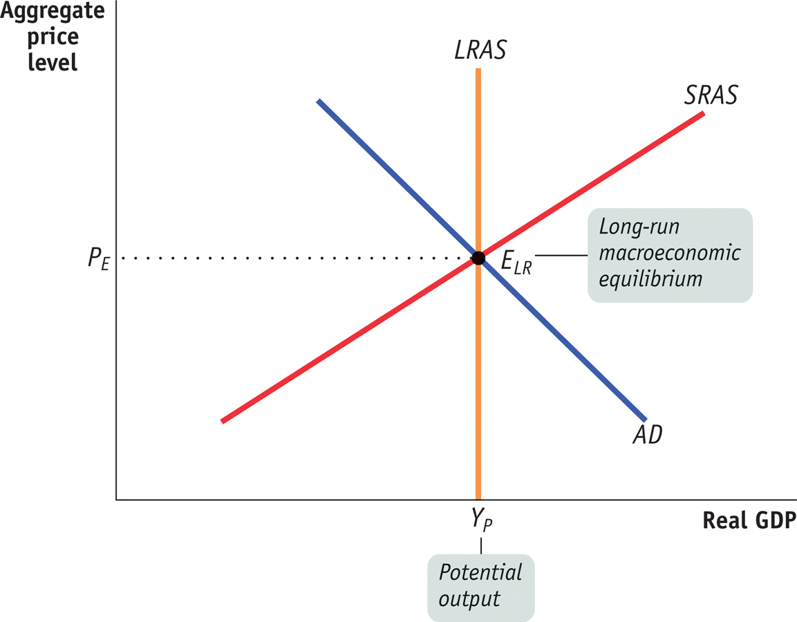
Long-Run Macroeconomic Equilibrium Here the point of short-run macroeconomic equilibrium also lies on the long-run aggregate supply curve, LRAS. As a result, short-run equilibrium aggregate output is equal to potential output, YP. The economy is in long-run macroeconomic equilibrium at ELR.
The economy is in long-run macroeconomic equilibrium when the point of short-run macroeconomic equilibrium is on the long-run aggregate supply curve.
To see the significance of long-run macroeconomic equilibrium, let’s consider what happens if a demand shock moves the economy away from long-run macroeconomic equilibrium. In Figure 12-15, we assume that the initial aggregate demand curve is AD1 and the initial short-run aggregate supply curve is SRAS1. So the initial macroeconomic equilibrium is at E1, which lies on the long-run aggregate supply curve, LRAS. The economy, then, starts from a point of short-run and long-run macroeconomic equilibrium, and short-run equilibrium aggregate output equals potential output at Y1.
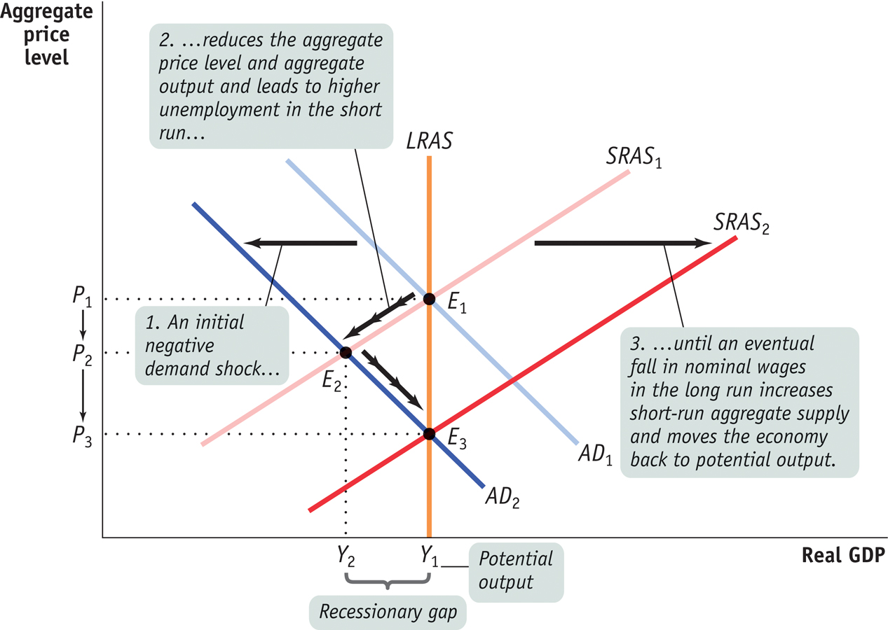
Short-Run versus Long-Run Effects of a Negative Demand Shock In the long run the economy is self-correcting: demand shocks have only a short-run effect on aggregate output. Starting at E1, a negative demand shock shifts AD1 leftward to AD2. In the short run the economy moves to E2 and a recessionary gap arises: the aggregate price level declines from P1 to P2, aggregate output declines from Y1 to Y2, and unemployment rises. But in the long run nominal wages fall in response to high unemployment at Y2, and SRAS1 shifts rightward to SRAS2. Aggregate output rises from Y2 to Y1, and the aggregate price level declines again, from P2 to P3. Long-run macroeconomic equilibrium is eventually restored at E3.
Now suppose that for some reason—such as a sudden worsening of business and consumer expectations—aggregate demand falls and the aggregate demand curve shifts leftward to AD2. This results in a lower equilibrium aggregate price level at P2 and a lower equilibrium aggregate output level at Y2 as the economy settles in the short run at E2. The short-run effect of such a fall in aggregate demand is what the U.S. economy experienced in 1929–1933: a falling aggregate price level and falling aggregate output.
There is a recessionary gap when aggregate output is below potential output.
Aggregate output in this new short-run equilibrium, E2, is below potential output. When this happens, the economy faces a recessionary gap. A recessionary gap inflicts a great deal of pain because it corresponds to high unemployment. The large recessionary gap that had opened up in the United States by 1933 caused intense social and political turmoil. And the devastating recessionary gap that opened up in Germany at the same time played an important role in Hitler’s rise to power.
But this isn’t the end of the story. In the face of high unemployment, nominal wages eventually fall, as do any other sticky prices, ultimately leading producers to increase output. As a result, a recessionary gap causes the short-run aggregate supply curve to gradually shift to the right over time. This process continues until SRAS1 reaches its new position at SRAS2, bringing the economy to equilibrium at E3, where AD2, SRAS2, and LRAS all intersect. At E3, the economy is back in long-run macroeconomic equilibrium; it is back at potential output Y1 but at a lower aggregate price level, P3, reflecting a long-run fall in the aggregate price level. In the end, the economy is self-correcting in the long run.
What if, instead, there was an increase in aggregate demand? The results are shown in Figure 12-16, where we again assume that the initial aggregate demand curve is AD1 and the initial short-run aggregate supply curve is SRAS1, so that the initial macroeconomic equilibrium, at E1, lies on the long-run aggregate supply curve, LRAS. Initially, then, the economy is in long-run macroeconomic equilibrium.
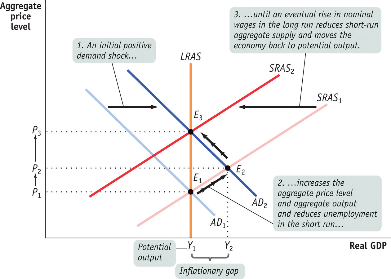
Short-Run versus Long-Run Effects of a Positive Demand Shock Starting at E1, a positive demand shock shifts AD1 rightward to AD2, and the economy moves to E2 in the short run. This results in an inflationary gap as aggregate output rises from Y1 to Y2, the aggregate price level rises from P1 to P2, and unemployment falls to a low level. In the long run, SRAS1 shifts leftward to SRAS2 as nominal wages rise in response to low unemployment at Y2. Aggregate output falls back to Y1, the aggregate price level rises again to P3, and the economy self-corrects as it returns to long-run macroeconomic equilibrium at E3.
There is an inflationary gap when aggregate output is above potential output.
Now suppose that aggregate demand rises, and the AD curve shifts rightward to AD2. This results in a higher aggregate price level, at P2, and a higher aggregate output level, at Y2, as the economy settles in the short run at E2. Aggregate output in this new short-run equilibrium is above potential output, and unemployment is low in order to produce this higher level of aggregate output. When this happens, the economy experiences an inflationary gap.
As in the case of a recessionary gap, this isn’t the end of the story. In the face of low unemployment, nominal wages will rise, as will other sticky prices. An inflationary gap causes the short-run aggregate supply curve to shift gradually to the left as producers reduce output in the face of rising nominal wages. This process continues until SRAS1 reaches its new position at SRAS2, bringing the economy to equilibrium at E3, where AD2, SRAS2, and LRAS all intersect. At E3, the economy is back in long-run macroeconomic equilibrium. It is back at potential output, but at a higher price level, P3, reflecting a long-run rise in the aggregate price level. Again, the economy is self-correcting in the long run.
Where’s the Deflation?
The AD–AS model says that either a negative demand shock or a positive supply shock should lead to a fall in the aggregate price level—that is, deflation. However, since 1949, an actual fall in the aggregate price level has been a rare occurrence in the United States. Similarly, most other countries have had little or no experience with deflation. Japan, which experienced sustained mild deflation in the late 1990s and the early part of the next decade, is the big (and much discussed) exception. What happened to deflation?
The basic answer is that since World War II economic fluctuations have largely taken place around a long-run inflationary trend. Before the war, it was common for prices to fall during recessions, but since then negative demand shocks have largely been reflected in a decline in the rate of inflation rather than an actual fall in prices. For example, the rate of consumer price inflation fell from more than 3% at the beginning of the 2001 recession to 1.1% a year later, but it never went below zero.
All of this changed during the recession of 2007–2009. The negative demand shock that followed the 2008 financial crisis was so severe that, for most of 2009, consumer prices in the United States indeed fell. But the deflationary period didn’t last long: beginning in 2010, prices again rose, at a rate of between 1% and 4% per year.
To summarize the analysis of how the economy responds to recessionary and inflationary gaps, we can focus on the output gap, the percentage difference between actual aggregate output and potential output. The output gap is calculated as follows:
The output gap is the percentage difference between actual aggregate output and potential output.
Our analysis says that the output gap always tends toward zero.
The economy is self-correcting when shocks to aggregate demand affect aggregate output in the short run, but not the long run.
If there is a recessionary gap, so that the output gap is negative, nominal wages eventually fall, moving the economy back to potential output and bringing the output gap back to zero. If there is an inflationary gap, so that the output gap is positive, nominal wages eventually rise, also moving the economy back to potential output and again bringing the output gap back to zero. So in the long run the economy is self-correcting: shocks to aggregate demand affect aggregate output in the short run but not in the long run.
!worldview! ECONOMICS in Action: Supply Shocks Versus Demand Shocks in Practice
Supply Shocks Versus Demand Shocks in Practice
How often do supply shocks and demand shocks, respectively, cause recessions? The verdict of most, though not all, macroeconomists is that recessions are mainly caused by demand shocks. But when a negative supply shock does happen, the resulting recession tends to be particularly severe.
Let’s get specific. Officially there have been twelve recessions in the United States since World War II. However, two of these, in 1979–1980 and 1981–1982, are often treated as a single “double-dip” recession, bringing the total number down to eleven. Of these eleven recessions, only two—the recession of 1973–1975 and the double-dip recession of 1979–1982—showed the distinctive combination of falling aggregate output and a surge in the price level that we call stagflation. In each case, the cause of the supply shock was political turmoil in the Middle East—the Arab–Israeli war of 1973 and the Iranian revolution of 1979—that disrupted world oil supplies and sent oil prices skyrocketing. In fact, economists sometimes refer to the two slumps as “OPEC I” and “OPEC II,” after the Organization of Petroleum Exporting Countries, the world oil cartel. A third recession that began in 2007 and lasted until 2009 was at least partially exacerbated, if not at least partially caused, by a spike in oil prices.
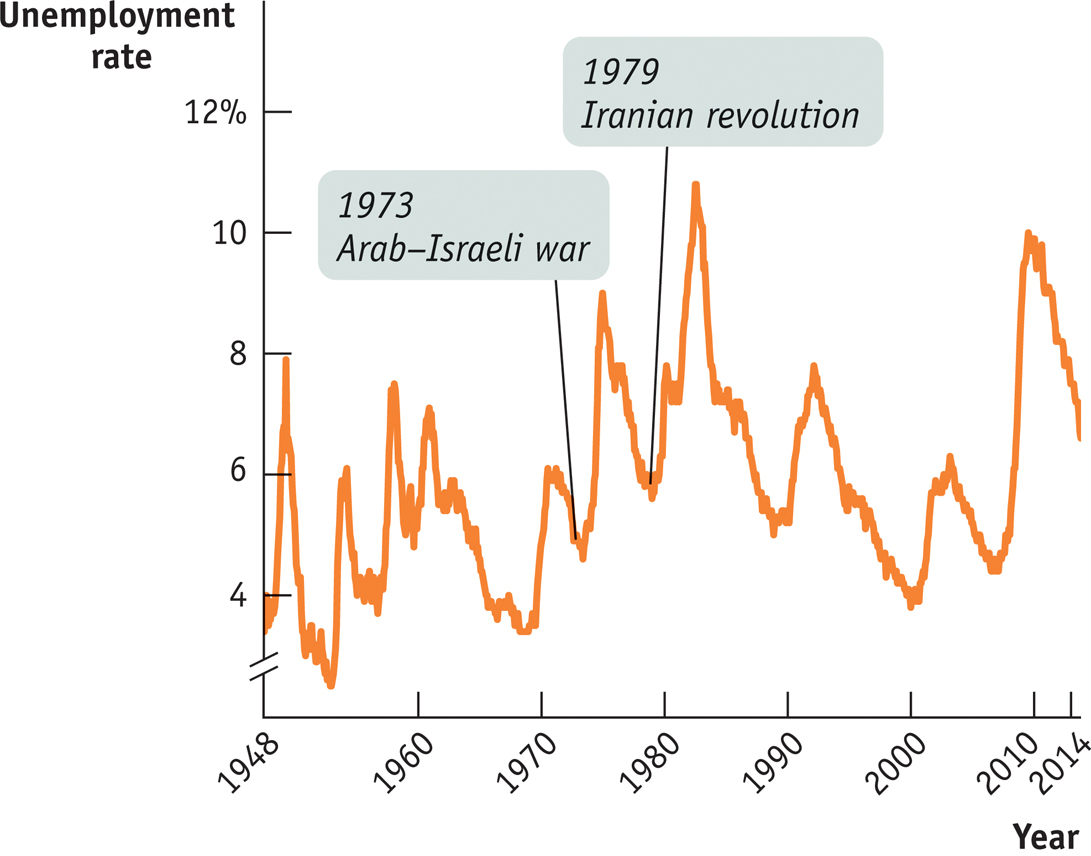
Negative Supply Shocks Are Relatively Rare but Nasty Source: Bureau of Labor Statistics.
So eight of eleven postwar recessions were purely the result of demand shocks, not supply shocks. The few supply-shock recessions, however, were the worst as measured by the unemployment rate. Figure 12-17 shows the U.S. unemployment rate since 1948, with the dates of the 1973 Arab–Israeli war and the 1979 Iranian revolution marked on the graph. Some of the highest unemployment rates since World War II came after these big negative supply shocks.
There’s a reason the aftermath of a supply shock tends to be particularly severe for the economy: macroeconomic policy has a much harder time dealing with supply shocks than with demand shocks. Indeed, the reason the Federal Reserve was having a hard time in 2008, as described in the opening story, was the fact that in early 2008 the U.S. economy was in a recession partially caused by a supply shock (although it was also facing a demand shock). We’ll see in a moment why supply shocks present such a problem.
Quick Review
The AD–AS model is used to study economic fluctuations.
Short-run macroeconomic equilibrium occurs at the intersection of the short-run aggregate supply and aggregate demand curves. This determines the short-run equilibrium aggregate price level and the level of short-run equilibrium aggregate output.
A demand shock, a shift of the AD curve, causes the aggregate price level and aggregate output to move in the same direction. A supply shock, a shift of the SRAS curve, causes them to move in opposite directions. Stagflation is the consequence of a negative supply shock.
A fall in nominal wages occurs in response to a recessionary gap, and a rise in nominal wages occurs in response to an inflationary gap. Both move the economy to long-run macroeconomic equilibrium, where the AD, SRAS, and LRAS curves intersect.
The output gap always tends toward zero because the economy is self-correcting in the long run.
12-3
Question
12.4
Describe the short-run effects of each of the following shocks on the aggregate price level and on aggregate output.
The government sharply increases the minimum wage, raising the wages of many workers.
Solar energy firms launch a major program of investment spending.
Congress raises taxes and cuts spending.
Severe weather destroys crops around the world.
Question
12.5
A rise in productivity increases potential output, but some worry that demand for the additional output will be insufficient even in the long run. How would you respond?
Solutions appear at back of book.
