The Aggregate Demand Curve and the Income–Expenditure Model
In the preceding chapter we introduced the income–expenditure model, which shows how the economy arrives at income–expenditure equilibrium. Now we’ve introduced the aggregate demand curve, which relates the overall demand for goods and services to the overall price level. How do these concepts fit together?
Recall that one of the assumptions of the income–expenditure model is that the aggregate price level is fixed. We now drop that assumption. We can still use the income–expenditure model, however, to ask what aggregate spending would be at any given aggregate price level, which is precisely what the aggregate demand curve shows. So the AD curve is actually derived from the income–expenditure model. Economists sometimes say that the income–expenditure model is “embedded” in the AD–AS model.
Figure 12-2 shows, once again, how income–expenditure equilibrium is determined. Real GDP is on the horizontal axis; real planned aggregate spending is on the vertical axis. Other things equal, planned aggregate spending, equal to consumer spending plus planned investment spending, rises with real GDP. This is illustrated by the upward-sloping lines  and
and  . Income–expenditure equilibrium, as we learned in Chapter 11, is at the point where the line representing planned aggregate spending crosses the 45-degree line. For example, if is the relationship between real GDP and planned aggregate spending, then income– expenditure equilibrium is at point E1, corresponding to a level of real GDP equal to Y1.
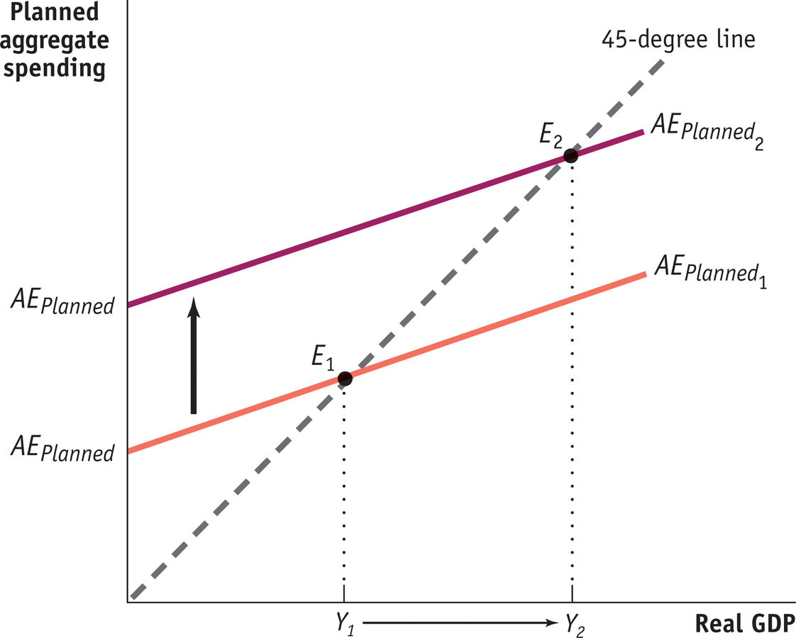
How Changes in the Aggregate Price Level Affect Income–Expenditure Equilibrium Income–expenditure equilibrium occurs at the point where the curve AEPlanned, which shows real aggregate planned spending, crosses the 45-degree line. A fall in the aggregate price level causes the AEPlanned curve to shift from to , leading to a rise in income–expenditure equilibrium GDP from Y1 to Y2.
We’ve just seen, however, that changes in the aggregate price level change the level of planned aggregate spending at any given level of real GDP. This means that when the aggregate price level changes, the AEPlanned curve shifts. For example, suppose that the aggregate price level falls. As a result of both the wealth effect and the interest rate effect, the fall in the aggregate price level will lead to higher planned aggregate spending at any given level of real GDP. So the AEPlanned curve will shift up, as illustrated in Figure 12-2 by the shift from to . The increase in planned aggregate spending leads to a multiplier process that moves the income–expenditure equilibrium from point E1 to point E2, raising real GDP from Y1 to Y2.
Figure 12-3 shows how this result can be used to derive the aggregate demand curve. In Figure 12-3, we show a fall in the aggregate price level from P1 to P2. We saw in Figure 12-2 that a fall in the aggregate price level would lead to an upward shift of the AEPlanned curve and hence a rise in real GDP. You can see this same result in Figure 12-3 as a movement along the AD curve: as the aggregate price level falls, real GDP rises from Y1 to Y2.
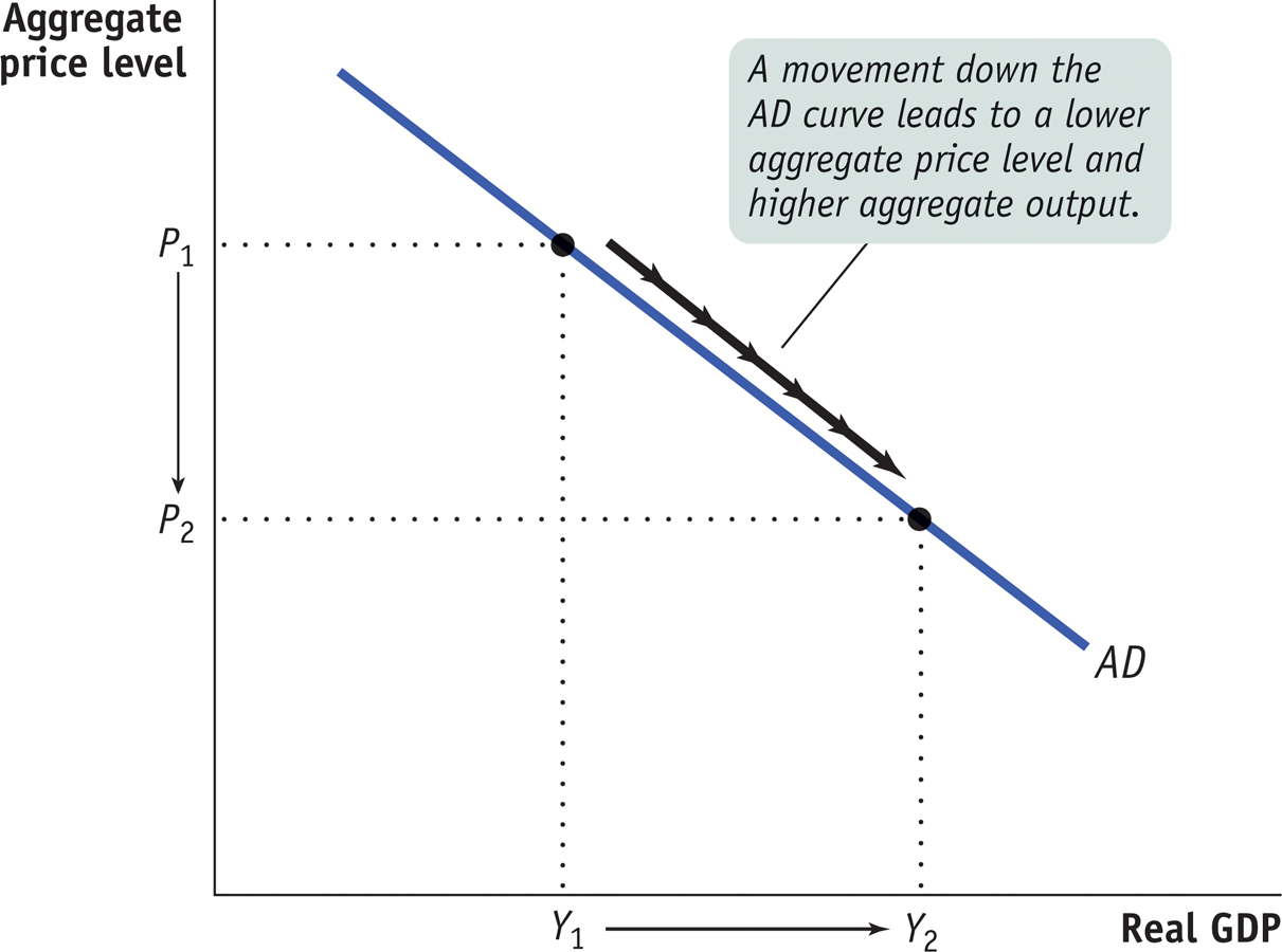
The Income–Expenditure Model and the Aggregate Demand Curve In Figure 12-2 we saw how a fall in the aggregate price level shifts the planned aggregate spending curve up, leading to a rise in real GDP. Here we show that same result as a movement along the aggregate demand curve. If the aggregate price level falls from P1 to P2, real GDP rises from Y1 to Y2. The AD curve is therefore downward sloping.
So the aggregate demand curve doesn’t replace the income–expenditure model. Instead, it’s a way to summarize what the income–expenditure model says about the effects of changes in the aggregate price level.
In practice, economists often use the income–expenditure model to analyze short-run economic fluctuations, even though strictly speaking it should be seen as a component of a more complete model. In the short run, in particular, this is usually a reasonable shortcut.