Shifts of the Short-Run Aggregate Supply Curve
Figure 12-5 shows a movement along the short-run aggregate supply curve, as the aggregate price level and aggregate output fell from 1929 to 1933. But there can also be shifts of the short-run aggregate supply curve, as shown in Figure 12-6. Panel (a) shows a decrease in short-run aggregate supply—a leftward shift of the short-run aggregate supply curve. Aggregate supply decreases when producers reduce the quantity of aggregate output they are willing to supply at any given aggregate price level. Panel (b) shows an increase in short-run aggregate supply—a rightward shift of the short-run aggregate supply curve. Aggregate supply increases when producers increase the quantity of aggregate output they are willing to supply at any given aggregate price level.

Shifts of the Short-Run Aggregate Supply Curve Panel (a) shows a decrease in short-run aggregate supply: the short-run aggregate supply curve shifts leftward from SRAS1 to SRAS2, and the quantity of aggregate output supplied at any given aggregate price level falls. Panel (b) shows an increase in short-run aggregate supply: the short-run aggregate supply curve shifts rightward from SRAS1 to SRAS2, and the quantity of aggregate output supplied at any given aggregate price level rises.
To understand why the short-run aggregate supply curve can shift, it’s important to recall that producers make output decisions based on their profit per unit of output. The short-run aggregate supply curve illustrates the relationship between the aggregate price level and aggregate output: because some production costs are fixed in the short run, a change in the aggregate price level leads to a change in producers’ profit per unit of output and, in turn, leads to a change in aggregate output. But other factors besides the aggregate price level can affect profit per unit and, in turn, aggregate output. It is changes in these other factors that will shift the short-run aggregate supply curve.
To develop some intuition, suppose that something happens that raises production costs—say, an increase in the price of oil. At any given price of output, a producer now earns a smaller profit per unit of output. As a result, producers reduce the quantity supplied at any given aggregate price level, and the short-run aggregate supply curve shifts to the left. If, in contrast, something happens that lowers production costs—say, a fall in the nominal wage—a producer now earns a higher profit per unit of output at any given price of output. This leads producers to increase the quantity of aggregate output supplied at any given aggregate price level, and the short-run aggregate supply curve shifts to the right.
Now we’ll discuss some of the important factors that affect producers’ profit per unit and so can lead to shifts of the short-run aggregate supply curve.
Changes in Commodity Prices In this chapter’s opening story, we described how a surge in the price of oil caused problems for the U.S. economy in the 1970s and early in 2008. Oil is a commodity, a standardized input bought and sold in bulk quantities. An increase in the price of a commodity—oil—raised production costs across the economy and reduced the quantity of aggregate output supplied at any given aggregate price level, shifting the short-run aggregate supply curve to the left. Conversely, a decline in commodity prices reduces production costs, leading to an increase in the quantity supplied at any given aggregate price level and a rightward shift of the short-run aggregate supply curve.
Why isn’t the influence of commodity prices already captured by the short-run aggregate supply curve? Because commodities—unlike, say, soft drinks—are not a final good, their prices are not included in the calculation of the aggregate price level. Further, commodities represent a significant cost of production to most suppliers, just like nominal wages do. So changes in commodity prices have large impacts on production costs. And in contrast to noncommodities, the prices of commodities can sometimes change drastically due to industry-specific shocks to supply—such as wars in the Middle East or rising Chinese demand that leaves less oil for the United States.
Changes in Nominal Wages At any given point in time, the dollar wages of many workers are fixed because they are set by contracts or informal agreements made in the past. Nominal wages can change, however, once enough time has passed for contracts and informal agreements to be renegotiated. Suppose, for example, that there is an economy-wide rise in the cost of health care insurance premiums paid by employers as part of employees’ wages. From the employers’ perspective, this is equivalent to a rise in nominal wages because it is an increase in employer-paid compensation. So this rise in nominal wages increases production costs and shifts the short-run aggregate supply curve to the left. Conversely, suppose there is an economy-wide fall in the cost of such premiums. This is equivalent to a fall in nominal wages from the point of view of employers; it reduces production costs and shifts the short-run aggregate supply curve to the right.
An important historical fact is that during the 1970s the surge in the price of oil had the indirect effect of also raising nominal wages. This “knock-on” effect occurred because many wage contracts included cost-of-living allowances that automatically raised the nominal wage when consumer prices increased. Through this channel, the surge in the price of oil—which led to an increase in overall consumer prices—ultimately caused a rise in nominal wages.
So the economy, in the end, experienced two leftward shifts of the aggregate supply curve: the first generated by the initial surge in the price of oil, the second generated by the induced increase in nominal wages. The negative effect on the economy of rising oil prices was greatly magnified through the cost-of-living allowances in wage contracts. Today, cost-of-living allowances in wage contracts are rare.
Changes in Productivity An increase in productivity means that a worker can produce more units of output with the same quantity of inputs. For example, the introduction of bar-code scanners in retail stores greatly increased the ability of a single worker to stock, inventory, and resupply store shelves. As a result, the cost to a store of “producing” a dollar of sales fell and profit rose. And, correspondingly, the quantity supplied increased. (Think of Walmart and the increase in the number of its stores as an increase in aggregate supply.) So a rise in productivity, whatever the source, increases producers’ profits and shifts the short-run aggregate supply curve to the right.
Conversely, a fall in productivity—say, due to new regulations that require workers to spend more time filling out forms—reduces the number of units of output a worker can produce with the same quantity of inputs. Consequently, the cost per unit of output rises, profit falls, and quantity supplied falls. This shifts the short-run aggregate supply curve to the left.
For a summary of the factors that shift the short-run aggregate supply curve, see Table 12-2.
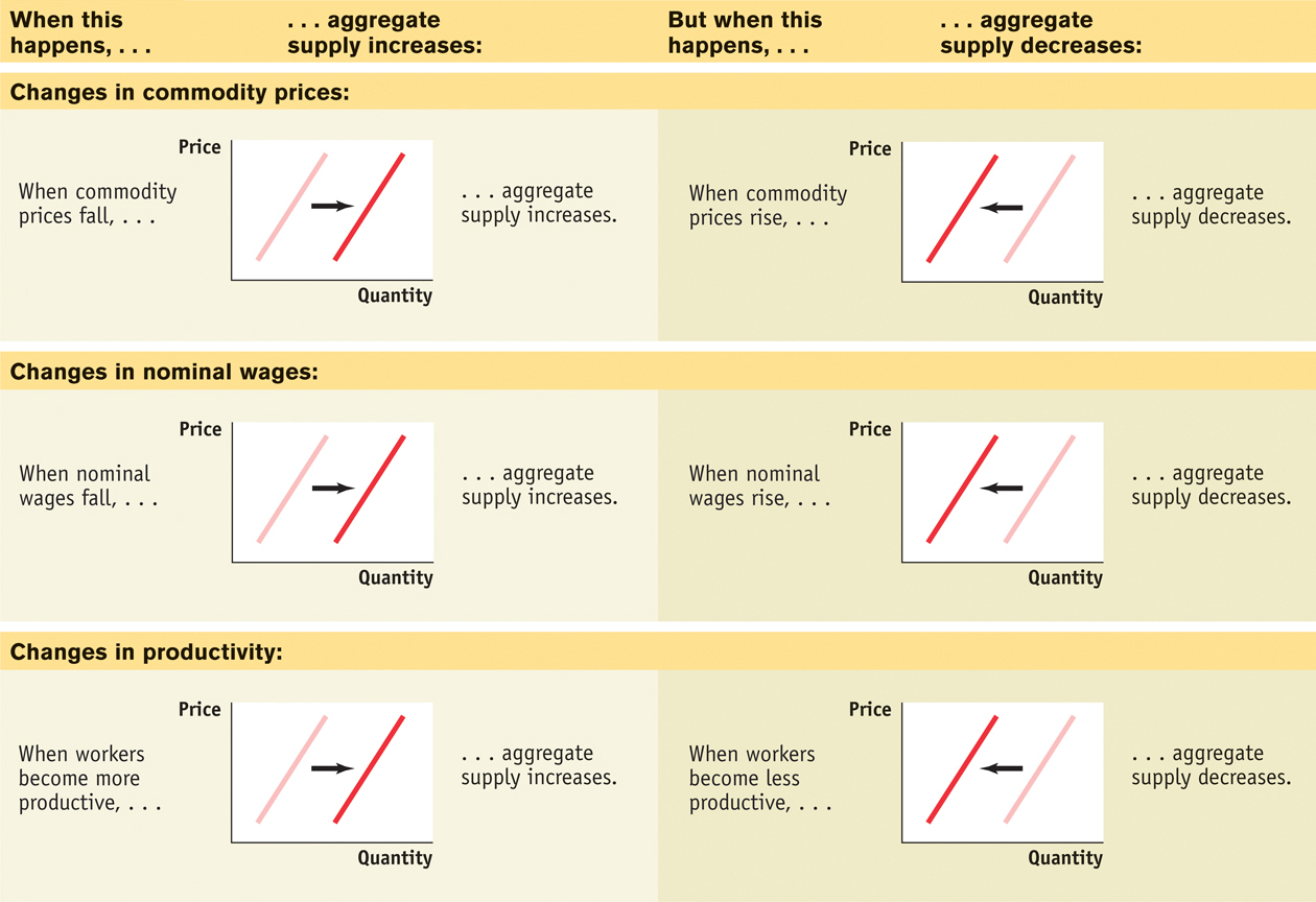
TABLE 12-2 Factors That Shift Aggregate Supply