Expansionary and Contractionary Fiscal Policy
Why would the government want to shift the aggregate demand curve? Because it wants to close either a recessionary gap, created when aggregate output falls below potential output, or an inflationary gap, created when aggregate output exceeds potential output.
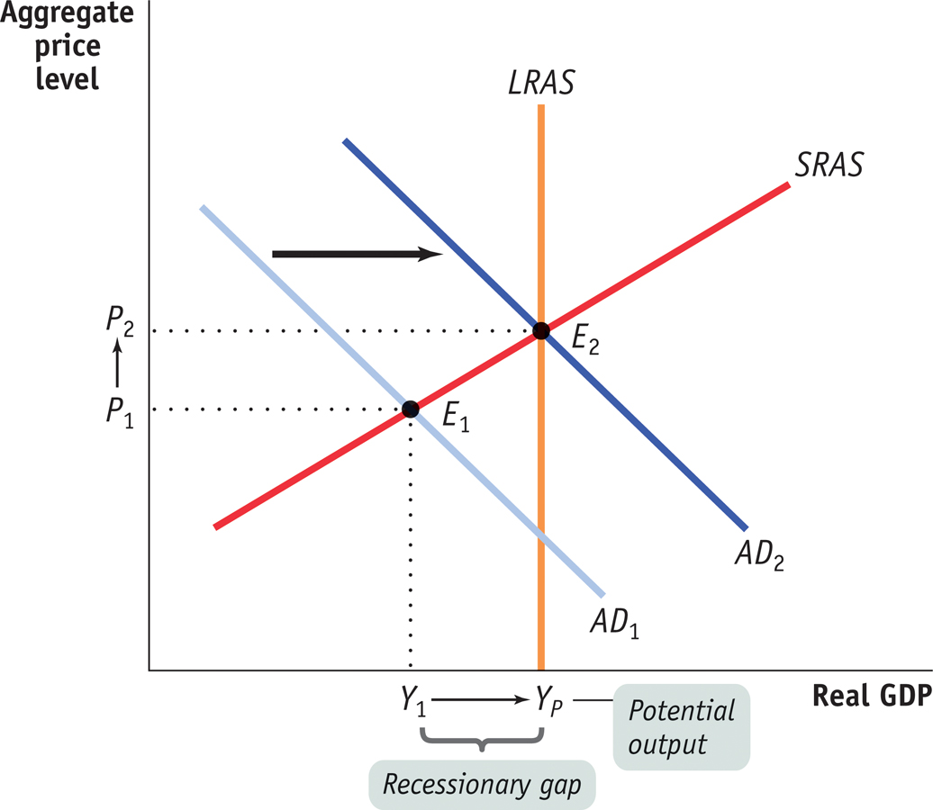
Figure 13-4 shows the case of an economy facing a recessionary gap. SRAS is the short-run aggregate supply curve, LRAS is the long-run aggregate supply curve, and AD1 is the initial aggregate demand curve. At the initial short-run macroeconomic equilibrium, E1, aggregate output is Y1, below potential output, YP. What the government would like to do is increase aggregate demand, shifting the aggregate demand curve rightward to AD2. This would increase aggregate output, making it equal to potential output. Fiscal policy that increases aggregate demand, called expansionary fiscal policy, normally takes one of three forms:
An increase in government purchases of goods and services
-
An increase in government transfers

Expansionary Fiscal Policy Can Close a Recessionary Gap The economy is in short-run macroeconomic equilibrium at E1, where the aggregate demand curve, AD1, intersects the SRAS curve. However, it is not in long-run macroeconomic equilibrium. At E1, there is a recessionary gap of YP − Y1. An expansionary fiscal policy—an increase in government purchases of goods and services, a reduction in taxes, or an increase in government transfers—shifts the aggregate demand curve rightward. It can close the recessionary gap by shifting AD1 to AD2, moving the economy to a new short-run macroeconomic equilibrium, E2, which is also a long-run macroeconomic equilibrium.
Expansionary fiscal policy is fiscal policy that increases aggregate demand.
The 2009 American Recovery and Reinvestment Act, or simply, the Recovery Act, was a combination of all three: a direct increase in federal spending and aid to state governments to help them maintain spending, tax cuts for most families, and increased aid to the unemployed.
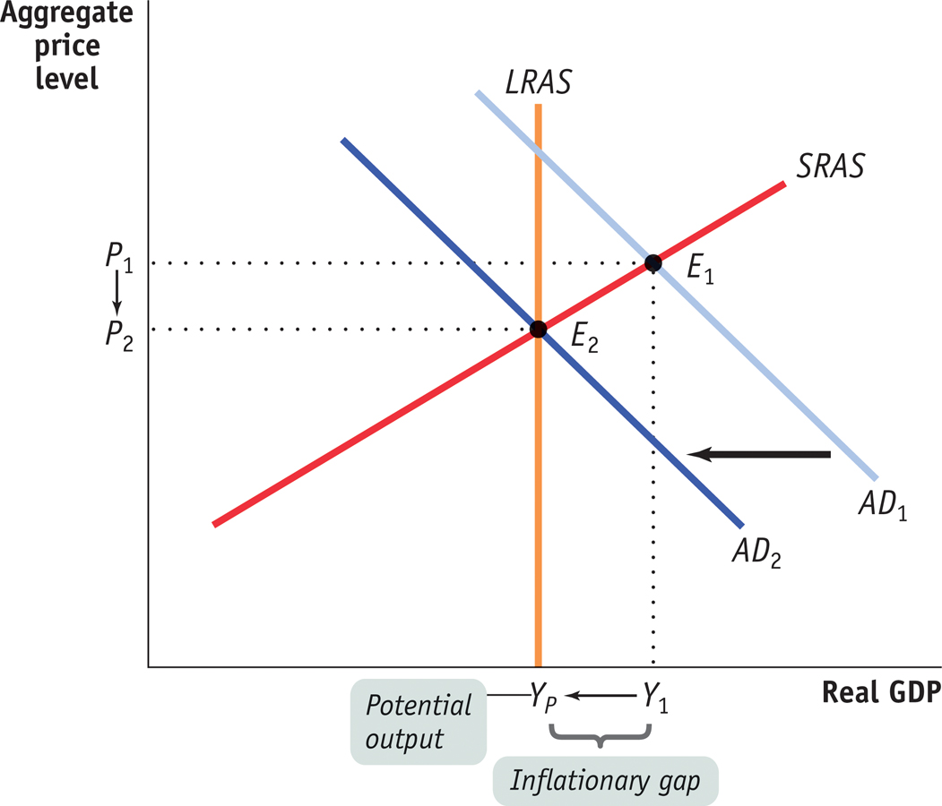
Figure 13-5 shows the opposite case—an economy facing an inflationary gap. Again, SRAS is the short-run aggregate supply curve, LRAS is the long-run aggregate supply curve, and AD1 is the initial aggregate demand curve. At the initial equilibrium, E1, aggregate output is Y1, above potential output, Yp. As we’ll explain in later chapters, policy makers often try to head off inflation by eliminating inflationary gaps. To eliminate the inflationary gap shown in Figure 13-5, fiscal policy must reduce aggregate demand and shift the aggregate demand curve leftward to AD2. This reduces aggregate output and makes it equal to potential output. Fiscal policy that reduces aggregate demand, called contractionary fiscal policy, is the opposite of expansionary fiscal policy. It is implemented in three possible ways:
A reduction in government purchases of goods and services
-
A reduction in government transfers

Contractionary Fiscal Policy Can Close an Inflationary Gap The economy is in short-run macroeconomic equilibrium at E1, where the aggregate demand curve, AD1, intersects the SRAS curve. But it is not in long-run macroeconomic equilibrium. At E1, there is an inflationary gap of Y1 Yp. A contractionary fiscal policy—such as reduced government purchases of goods and services, an increase in taxes, or a reduction in government transfers—shifts the aggregate demand curve leftward. It closes the inflationary gap by shifting AD1 to AD2, moving the economy to a new short-run macroeconomic equilibrium, E2, which is also a long-run macroeconomic equilibrium.
Contractionary fiscal policy is fiscal policy that reduces aggregate demand.
A classic example of contractionary fiscal policy occurred in 1968, when U.S. policy makers grew worried about rising inflation. President Lyndon Johnson imposed a temporary 10% surcharge on taxable income—everyone’s income taxes were increased by 10%. He also tried to scale back government purchases of goods and services, which had risen dramatically because of the cost of the Vietnam War.

