1.3 29The AD–AS Model

WHAT YOU WILL LEARN
 The difference between short-
run and long- run macroeconomic equilibrium  The causes and effects of demand shocks and supply shocks
 How to determine if an economy is experiencing a recessionary gap or an inflationary gap and how to calculate the size of output gaps
 How monetary policy and fiscal policy can be used to stabilize the economy
Putting the Aggregate Supply Curve and the Aggregate Demand Curve Together
From 1929 to 1933, the U.S. economy moved down the short-
In the AD–
So to understand the behavior of the economy, we must put the aggregate supply curve and the aggregate demand curve together. The result is the AD–
Short-Run Macroeconomic Equilibrium
The economy is in short-
The short-
Short-
We’ll begin our analysis by focusing on the short run. Figure 29-1 shows the aggregate demand curve and the short-
![FIGURE 29-1 The [em]AD–AS[/em] Model](asset/Sec08/c29_fig01.jpg)
We have seen that a shortage of any individual good causes its market price to rise and a surplus of the good causes its market price to fall. These forces ensure that the market reaches equilibrium. The same logic applies to short-
If the aggregate price level is below its equilibrium level, the quantity of aggregate output supplied is less than the quantity of aggregate output demanded. This leads to a rise in the aggregate price level, again pushing it toward its equilibrium level. In the discussion that follows, we’ll assume that the economy is always in short-
We’ll also make another important simplification based on the observation that in reality there is a long-
In fact, since the Great Depression there have been very few years in which the aggregate price level of any major nation actually declined—
The short-
Shifts of Aggregate Demand: Short-Run Effects
An event that shifts the aggregate demand curve is a demand shock.
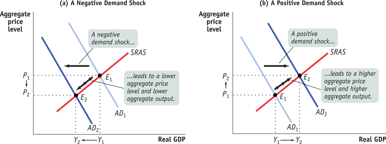
An event that shifts the aggregate demand curve, such as a change in expectations or wealth, the effect of the size of the existing stock of physical capital, or the use of fiscal or monetary policy, is known as a demand shock. The Great Depression was caused by a negative demand shock—
Figure 29-2 shows the short-
Shifts of the SRAS Curve
An event that shifts the short-
An event that shifts the short-
In contrast, a positive supply shock reduces production costs and increases the quantity supplied at any given aggregate price level, leading to a rightward shift of the short-
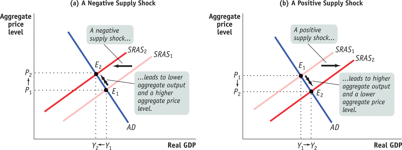
The effects of a negative supply shock are shown in panel (a) of Figure 29-3. The initial equilibrium is at E1, with aggregate price level P1 and aggregate output Y1. The disruption in the oil supply causes the short-
Stagflation is the combination of inflation and stagnating (or falling) aggregate output.
The combination of inflation and falling aggregate output shown in panel (a) has a special name: stagflation, for “stagnation plus inflation.” When an economy experiences stagflation, it’s very unpleasant: falling aggregate output leads to rising unemployment, and people feel that their purchasing power is squeezed by rising prices. Stagflation in the 1970s led to a mood of national pessimism. It also, as we’ll see shortly, poses a dilemma for policy makers.
A positive supply shock, shown in panel (b), has exactly the opposite effects. A rightward shift of the SRAS curve, from SRAS1 to SRAS2, results in a rise in aggregate output and a fall in the aggregate price level, a downward movement along the AD curve. The favorable supply shocks of the late 1990s led to a combination of full employment and declining inflation. That is, the aggregate price level fell compared with the long-

The distinctive feature of supply shocks, both negative and positive, is that, unlike demand shocks, they cause the aggregate price level and aggregate output to move in opposite directions.
There’s another important contrast between supply shocks and demand shocks. As we’ve seen, monetary policy and fiscal policy enable the government to shift the aggregate demand curve, meaning that governments are in a position to create the kinds of shocks shown in Figure 29-2. It’s much harder for governments to shift the aggregate supply curve. Are there good policy reasons to shift the aggregate demand curve? We’ll turn to that question soon. First, however, let’s look at the difference between short-
Long-Run Macroeconomic Equilibrium
The economy is in long-
Figure 29-4 combines the aggregate demand curve with both the short-
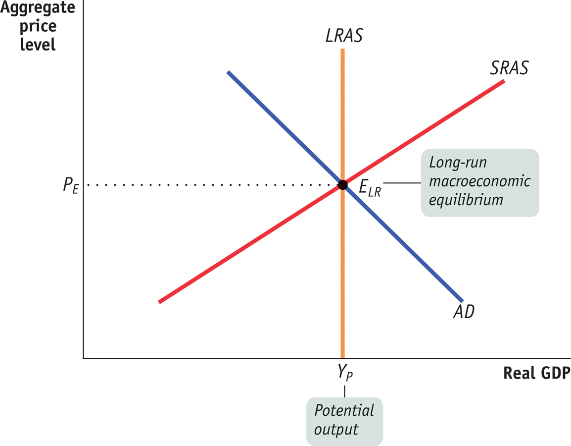
To see the significance of long-
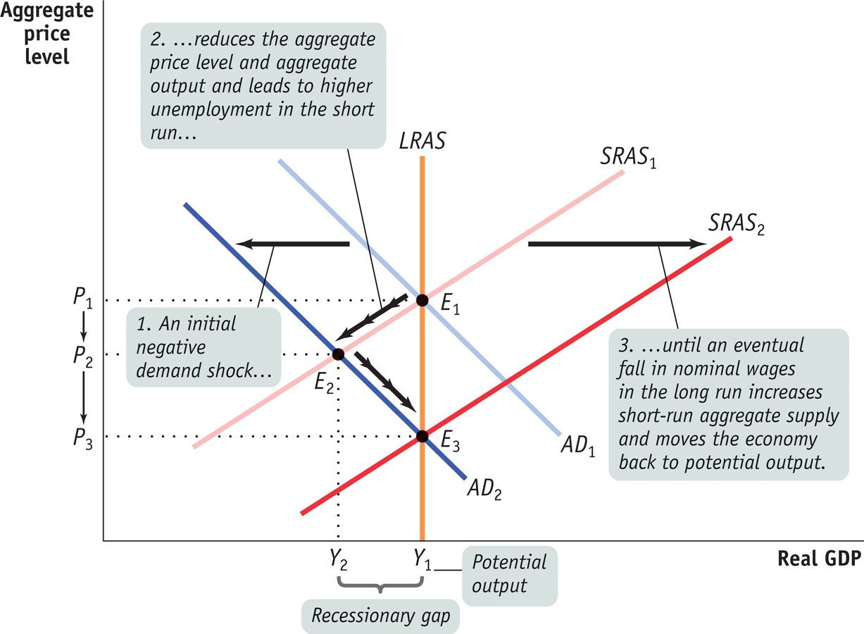
Now suppose that for some reason—
There is a recessionary gap when aggregate output is below potential output.
Aggregate output in this new short-

But this isn’t the end of the story. In the face of high unemployment, nominal wages eventually fall, as do any other sticky prices, ultimately leading producers to increase output. As a result, a recessionary gap causes the short-
What if, instead, there was an increase in aggregate demand? The results are shown in Figure 29-6, where we again assume that the initial aggregate demand curve is AD1 and the initial short-
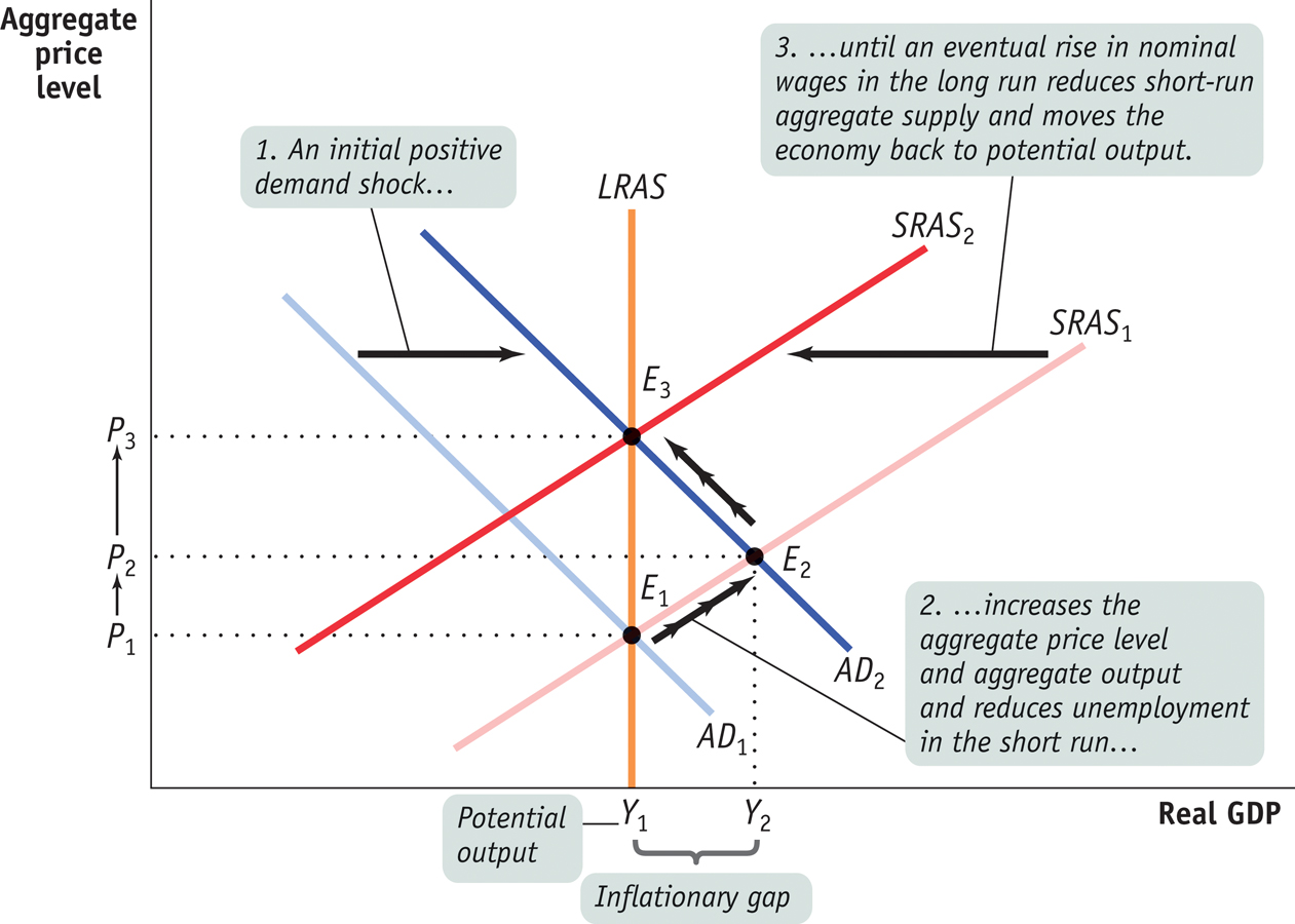
There is an inflationary gap when aggregate output is above potential output.
Now suppose that aggregate demand rises, and the AD curve shifts rightward to AD2. This results in a higher aggregate price level, at P2, and a higher aggregate output level, at Y2, as the economy settles in the short run at E2. Aggregate output in this new short-
In the face of low unemployment, nominal wages will rise, as will other sticky prices. An inflationary gap causes the short-
To summarize the analysis of how the economy responds to recessionary and inflationary gaps, we can focus on the output gap, the percentage difference between actual aggregate output and potential output. The output gap is calculated as follows:
The output gap is the percentage difference between actual aggregate output and potential output.

Our analysis says that the output gap always tends toward zero.
The economy is self-
If there is a recessionary gap, so that the output gap is negative, nominal wages eventually fall, moving the economy back to potential output and bringing the output gap back to zero. If there is an inflationary gap, so that the output gap is positive, nominal wages eventually rise, also moving the economy back to potential output and again bringing the output gap back to zero. So in the long run the economy is self-
SUPPLY SHOCKS VERSUS DEMAND SHOCKS IN PRACTICE
How often do supply shocks and demand shocks, respectively, cause recessions? The verdict of most, though not all, macroeconomists is that recessions are mainly caused by demand shocks. But when a negative supply shock does happen, the resulting recession tends to be particularly severe.
Let’s get specific. Officially there have been twelve recessions in the United States since World War II. However, two of these, in 1979–
In each case, the cause of the supply shock was political turmoil in the Middle East—
So eight of eleven postwar recessions were purely the result of demand shocks, not supply shocks. The few supply-
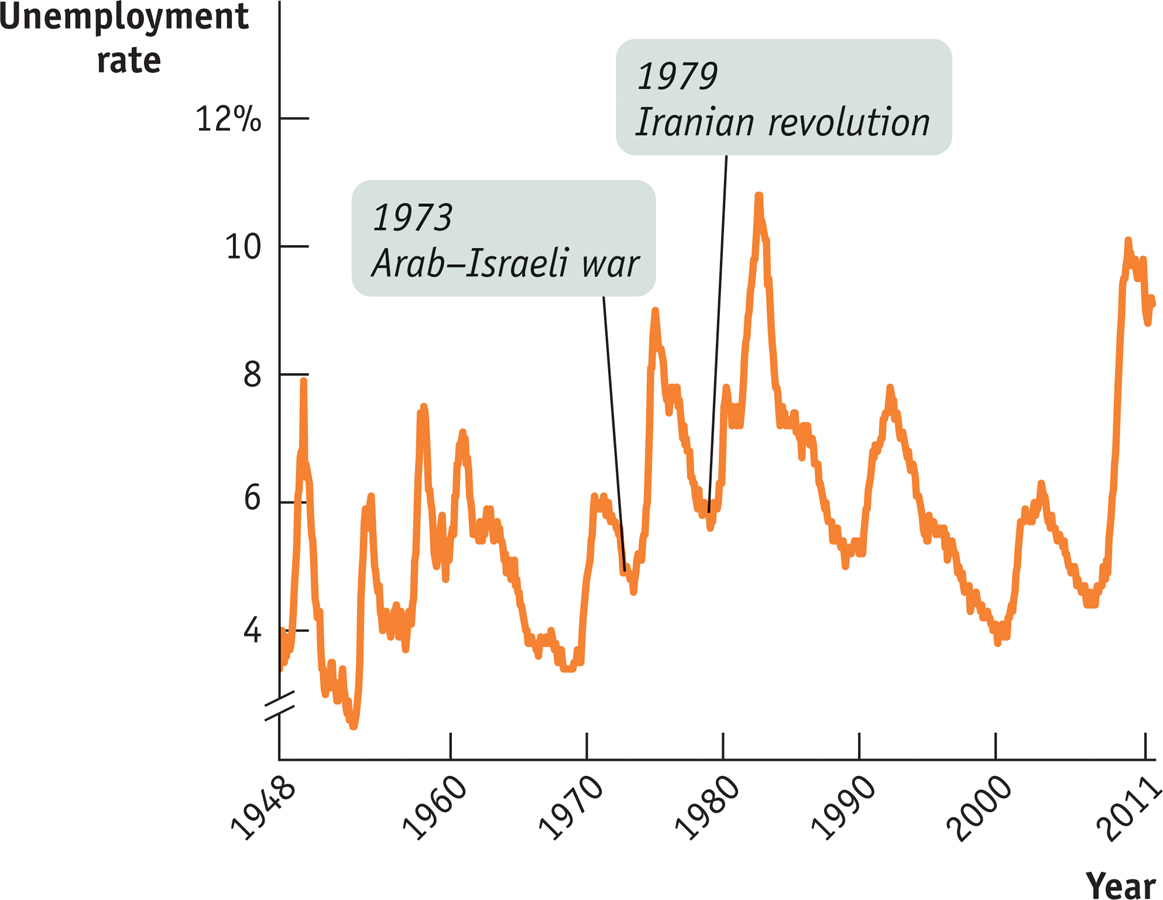
There’s a reason the aftermath of a supply shock tends to be particularly severe for the economy: macroeconomic policy has a much harder time dealing with supply shocks than with demand shocks. Indeed, the reason the Federal Reserve was having a hard time in 2008, as described in the section-
Macroeconomic Policy
We’ve just seen that the economy is self-
Most macroeconomists believe, however, that the process of self-
This belief is the background to one of the most famous quotations in economics: John Maynard Keynes’s declaration, “In the long run we are all dead.” Economists usually interpret Keynes as having recommended that governments not wait for the economy to correct itself. Instead, it is argued by many economists, but not all, that the government should use fiscal policy to get the economy back to potential output in the aftermath of a shift of the aggregate demand curve.
Stabilization policy is the use of government policy to reduce the severity of recessions and rein in excessively strong expansions.
This is the rationale for active stabilization policy, which is the use of government policy to reduce the severity of recessions and rein in excessively strong expansions.
Can stabilization policy improve the economy’s performance? As we saw in Figure 28-4, the answer certainly appears to be yes. Under active stabilization policy, the U.S. economy returned to potential output in 1996 after an approximately five-
Policy in the Face of Demand Shocks
Imagine that the economy experiences a negative demand shock, like the one shown by the shift from AD1 to AD2 in Figure 29-5. As we know, fiscal policy shifts the aggregate demand curve. If policy makers react quickly to the fall in aggregate demand, they can use monetary or fiscal policy to shift the aggregate demand curve back to the right. And if policy were able to perfectly anticipate shifts of the aggregate demand curve and counteract them, it could short-
Why might a policy that short-
Does this mean that policy makers should always act to offset declines in aggregate demand? Not necessarily. Some policy measures to increase aggregate demand, especially those that increase budget deficits, may have long-
Furthermore, in the real world policy makers aren’t perfectly informed, and the effects of their policies aren’t perfectly predictable. This creates the danger that stabilization policy will do more harm than good; that is, attempts to stabilize the economy may end up creating more instability. We’ll describe the long-
Should policy makers also try to offset positive shocks to aggregate demand? It may not seem obvious that they should. After all, even though inflation may be a bad thing, isn’t more output and lower unemployment a good thing? Again, not necessarily. Most economists now believe that any short-
Responding to Supply Shocks
In panel (a) of Figure 29-3 we showed the effects of a negative supply shock: in the short run such a shock leads to lower aggregate output but a higher aggregate price level. As we’ve noted, policy makers can respond to a negative demand shock by using monetary and fiscal policy to return aggregate demand to its original level. But what can or should they do about a negative supply shock?
In contrast to the case of a demand shock, there are no easy remedies for a supply shock. That is, there are no government policies that can easily counteract the changes in production costs that shift the short-

And if you consider using monetary or fiscal policy to shift the aggregate demand curve in response to a supply shock, the right response isn’t obvious.
Two bad things are happening simultaneously: a fall in aggregate output, leading to a rise in unemployment, and a rise in the aggregate price level. Any policy that shifts the aggregate demand curve helps one problem only by making the other worse. If the government acts to increase aggregate demand and limit the rise in unemployment, it reduces the decline in output but causes even more inflation. If it acts to reduce aggregate demand, it curbs inflation but causes a further rise in unemployment.
It’s a trade-
29
Solutions appear at the back of the book.
Check Your Understanding
Describe the short-
run effects of each of the following shocks on the aggregate price level and on aggregate output. -
a. The government sharply increases the minimum wage, raising the wages of many workers.
An increase in the minimum wage raises the nominal wage and, as a result, shifts the short-run aggregate supply curve to the left. As a result of this negative supply shock, the aggregate price level rises and aggregate output falls. -
b. Solar energy firms launch a major program of investment spending.
Increased investment spending shifts the aggregate demand curve to the right. As a result of this positive demand shock, both the aggregate price level and aggregate output rise. -
c. Congress raises taxes and cuts spending.
An increase in taxes and a reduction in government spending both result in negative demand shocks, shifting the aggregate demand curve to the left. As a result, both the aggregate price level and aggregate output fall. -
d. Severe weather destroys crops around the world.
This is a negative supply shock, shifting the short-run aggregate supply curve to the left. As a result, the aggregate price level rises and aggregate output falls.
-
A rise in productivity increases potential output, but some worry that demand for the additional output will be insufficient even in the long run. How would you respond?
As long-run growth increases potential output, the long-run aggregate supply curve shifts to the right. If, in the short run, there is now a recessionary gap (aggregate output is less than potential output), nominal wages will fall, shifting the short-run aggregate supply curve to the right. This results in a fall in the aggregate price level and a rise in aggregate output. As prices fall, we move along the aggregate demand curve due to the wealth and interest rate effects of a change in the aggregate price level. Eventually, as long-run macroeconomic equilibrium is reestablished, aggregate output will rise to be equal to potential output, and the aggregate price level will fall to the level that equates the quantity of aggregate output demanded with potential output.Suppose someone says, “Using monetary or fiscal policy to pump up the economy is counterproductive—
you get a brief high, but then you have the pain of inflation.” -
a. Explain what this means in terms of the AD–
AS model.An economy is overstimulated when an inflationary gap is present. This will arise if an expansionary monetary or fiscal policy is implemented when the economy is currently in long-run macroeconomic equilibrium. This shifts the aggregate demand curve to the right, in the short run raising the aggregate price level and aggregate output and creating an inflationary gap. Eventually nominal wages will rise and shift the short-run aggregate supply curve to the left, and aggregate output will fall back to potential output. This is the scenario envisaged by the speaker. -
b. Is this a valid argument against stabilization policy? Why or why not?
No, this is not a valid argument. When the economy is not currently in long-run macroeconomic equilibrium, an expansionary monetary or fiscal policy does not lead to the outcome described. Suppose a negative demand shock has shifted the aggregate demand curve to the left, resulting in a recessionary gap. An expansionary monetary or fiscal policy can shift the aggregate demand curve back to its original position in long-run macroeconomic equilibrium. In this way, the short-run fall in aggregate output and deflation caused by the original negative demand shock can be avoided. So, if used in response to demand shocks, fiscal or monetary policy is an effective policy tool.
-
In 2008, in the aftermath of the collapse of the housing bubble and a sharp rise in the price of commodities, particularly oil, there was much internal disagreement within the Fed about how to respond, with some advocating lowering interest rates and others contending that this would set off a rise in inflation. Explain the reasoning behind each of these views in terms of the AD–
AS model.Those within the Fed who advocated lowering interest rates were focused on boosting aggregate demand in order to counteract the negative demand shock caused by the collapse of the housing bubble. Lowering interest rates will result in a rightward shift of the aggregate demand curve, increasing aggregate output but raising the aggregate price level. Those within the Fed who advocated holding interest rates steady were focused on the fact that fighting the slump in aggregate demand in the face of a negative supply shock could result in a rise in inflation. Holding interest rates steady relies on the ability of the economy to self-correct in the long run, with the aggregate price level and aggregate output only gradually returning to their levels before the negative supply shock.
Multiple-
Question
Which of the following causes a negative supply shock?
I. a technological advance
II. increasing productivity
III. an increase in oil pricesA. B. C. D. E. Question
Which of the following causes a positive demand shock?
A. B. C. D. E. Question
During stagflation, what happens to the aggregate price level and real GDP?
Aggregate price levelReal GDPA. B. C. D. E.
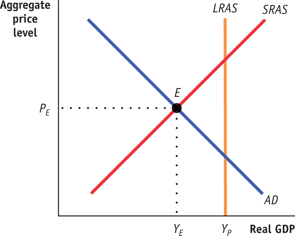
Refer to the graph for questions 4 and 5.
Question
Which of the following statements is true if this economy is operating at PE and YE?
I. The level of aggregate output equals potential output.
II. It is in short-run macroeconomic equilibrium.
III. It is in long-run macroeconomic equilibrium. A. B. C. D. E. Question
The economy depicted in the graph is experiencing a(n)
A. B. C. D. E.
Critical-
Question 1.2
Draw a graph to illustrate an economy in the midst of an inflationary gap. Explain and illustrate why the economy will eventually return to long-
Since output Y1 is above potential output, there is an inflationary gap. The low level of unemployment will cause nominal wages to rise, causing production cost to rise. This will shift the SRAS curve up and to the left. As the price level rises, there is a movement along the AD curve and output returns to its potential level.

WHERE’S THE DEFLATION?
 The AD–
 Rarely. Since 1949, an actual fall in the aggregate price level has been a rare occurrence in the United States. Similarly, most other countries have had little or no experience with deflation. Japan, which experienced sustained mild deflation in the late 1990s and the early part of the next decade, is the big (and much discussed) exception. What happened to deflation?
The basic answer is that since World War II economic fluctuations have largely taken place around a long-
To learn more, see pages 297–
