In an economy with no government and no foreign trade, there are only two sources of aggregate spending: consumer spending, C, and investment spending, I. And since we assume that there are no taxes or transfers, aggregate disposable income is equal to GDP (which, since the aggregate price level is fixed, is the same as real GDP): the total value of final sales of goods and services ultimately accrues to households as income. So in this highly simplified economy, there are two basic equations of national income accounting:

As we learned earlier in this chapter, the aggregate consumption function shows the relationship between disposable income and consumer spending. Let’s continue to assume that the aggregate consumption function is of the same form as in Equation 11-9:

In our simplified model, we will also assume planned investment spending, I_Planned, is fixed.

We need one more concept before putting the model together: planned aggregate spending, the total amount of planned spending in the economy. Unlike firms, households don’t take unintended actions like unplanned inventory investment. So planned aggregate spending is equal to the sum of consumer spending and planned investment spending. We denote planned aggregate spending by AE_Planned, so:

The level of planned aggregate spending in a given year depends on the level of real GDP in that year. To see why, let’s look at a specific example, shown in Table 11-2. We assume that the aggregate consumption function is:

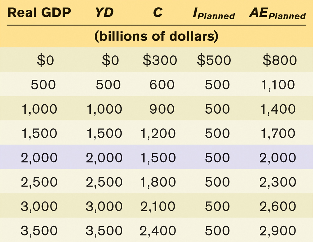
Real GDP, YD, C, I_Planned, and AE_Planned are all measured in billions of dollars, and we assume that the level of planned investment, I_Planned, is fixed at $500 billion per year. The first column shows possible levels of real GDP. The second column shows disposable income, YD, which in our simplified model is equal to real GDP. The third column shows consumer spending, C, equal to $300 billion plus 0.6 times disposable income, YD. The fourth column shows planned investment spending, I_Planned, which we have assumed is $500 billion regardless of the level of real GDP. Finally, the last column shows planned aggregate spending, AE_Planned, the sum of aggregate consumer spending, C, and planned investment spending, I_Planned. (To economize on notation, we’ll assume that it is understood from now on that all the variables in Table 11-2 are measured in billions of dollars per year.) As you can see, a higher level of real GDP leads to a higher level of disposable income: every 500 increase in real GDP raises YD by 500, which in turn raises C by 500 × 0.6 = 300 and AE_Planned by 300.

Figure 11-9 illustrates the information in Table 11-2 graphically. Real GDP is measured on the horizontal axis. CF is the aggregate consumption function; it shows how consumer spending depends on real GDP. AE_Planned, the planned aggregate spending line, corresponds to the aggregate consumption function shifted up by 500 (the amount of I_Planned). It shows how planned aggregate spending depends on real GDP. Both lines have a slope of 0.6, equal to MPC, the marginal propensity to consume.

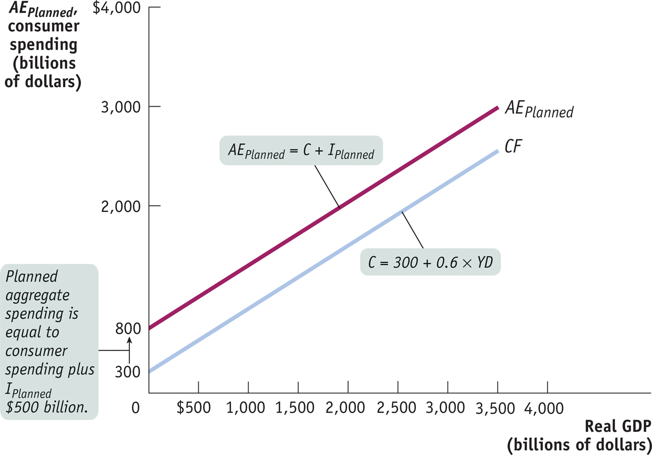
But this isn’t the end of the story. Table 11-2 reveals that real GDP equals planned aggregate spending, AE_Planned, only when the level of real GDP is at 2,000. Real GDP does not equal AE_Planned at any other level. Is that possible? Didn’t we learn in Chapter 7, with the circular-flow diagram, that total spending on final goods and services in the economy is equal to the total value of output of final goods and services? The answer is that for brief periods of time, planned aggregate spending can differ from real GDP because of the role of unplanned aggregate spending—I_Unplanned, unplanned inventory investment.

But as we’ll see in the next section, the economy moves over time to a situation in which there is no unplanned inventory investment, a situation called income–expenditure equilibrium. And when the economy is in income–expenditure equilibrium, planned aggregate spending on final goods and services equals aggregate output.