Current Disposable Income and Consumer Spending
The most important factor affecting a family’s consumer spending is its current disposable income—income after taxes are paid and government transfers are received. It’s obvious from daily life that people with high disposable incomes on average drive more expensive cars, live in more expensive houses, and spend more on meals and clothing than people with lower disposable incomes. And the relationship between current disposable income and spending is clear in the data.
The Bureau of Labor Statistics (BLS) collects annual data on family income and spending. Families are grouped by levels of before-tax income, and after-tax income for each group is also reported. Since the income figures include transfers from the government, what the BLS calls a household’s after-tax income is equivalent to its current disposable income.
Figure 11-2 is a scatter diagram illustrating the relationship between household current disposable income and household consumer spending for American households by income group in 2013. For example, point A shows that in 2013 the middle fifth of the population had an average current disposable income of $45,826 and average spending of $42,495. The pattern of the dots slopes upward from left to right, making it clear that households with higher current disposable income had higher consumer spending.
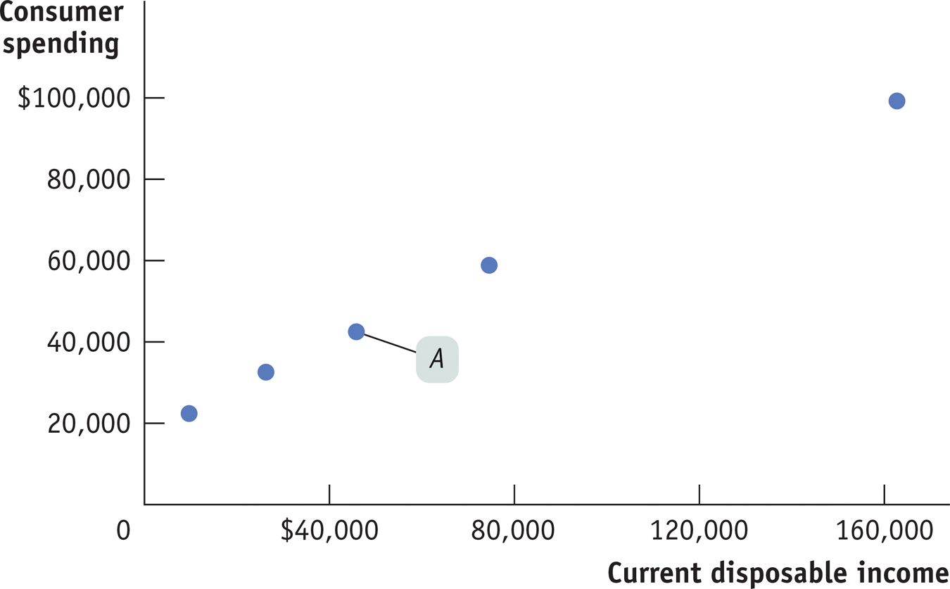
Current Disposable Income and Consumer Spending for American Households in 2013 For each income group of households, average current disposable income in 2012 is plotted versus average consumer spending in 2013. For example, the middle income group, with current disposable income of $40,187 to $65,501, is represented by point A, indicating a household average current disposable income of $45,826 and average household consumer spending of $42,495. The data clearly show a positive relationship between current disposable income and consumer spending: families with higher current disposable income have higher consumer spending. Source: Bureau of Labor Statistics.

During recessions, consumers tend to avoid higher-priced brand-name goods in favor of generics that cost less.
It’s very useful to represent the relationship between an individual household’s current disposable income and its consumer spending with an equation. The consumption function is an equation showing how an individual household’s consumer spending varies with the household’s current disposable income. The simplest version of a consumption function is a linear equation:
The consumption function is an equation showing how an individual household’s consumer spending varies with the household’s current disposable income.
where lowercase letters indicate variables measured for an individual household.
In this equation, c is individual household consumer spending and yd is individual household current disposable income. Recall that MPC, the marginal propensity to consume, is the amount by which consumer spending rises if current disposable income rises by $1. Finally, a is a constant term—individual household autonomous consumer spending, the amount of spending a household would do if it had zero disposable income. We assume that a is greater than zero because a household with zero disposable income is able to fund some consumption by borrowing or using its savings. Notice, by the way, that we’re using y for income. That’s standard practice in macroeconomics, even though income isn’t actually spelled “yncome.” The reason is that I is reserved for investment spending.
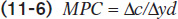
Recall that we expressed MPC as the ratio of a change in consumer spending to the change in current disposable income. We’ve rewritten it for an individual household as Equation 11-6:
Multiplying both sides of Equation 11-6 by Δyd, we get:
Equation 11-7 tells us that when yd goes up by $1, c goes up by MPC × $1.
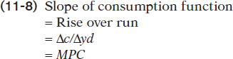
Figure 11-3 shows what Equation 11-5 looks like graphically, plotting yd on the horizontal axis and c on the vertical axis. Individual household autonomous consumer spending, a, is the value of c when yd is zero—it is the vertical intercept of the consumption function, cf. MPC is the slope of the line, measured by rise over run. If current disposable income rises by Δyd, household consumer spending, c, rises by Δc. Since MPC is defined as Δc/Δyd, the slope of the consumption function is:
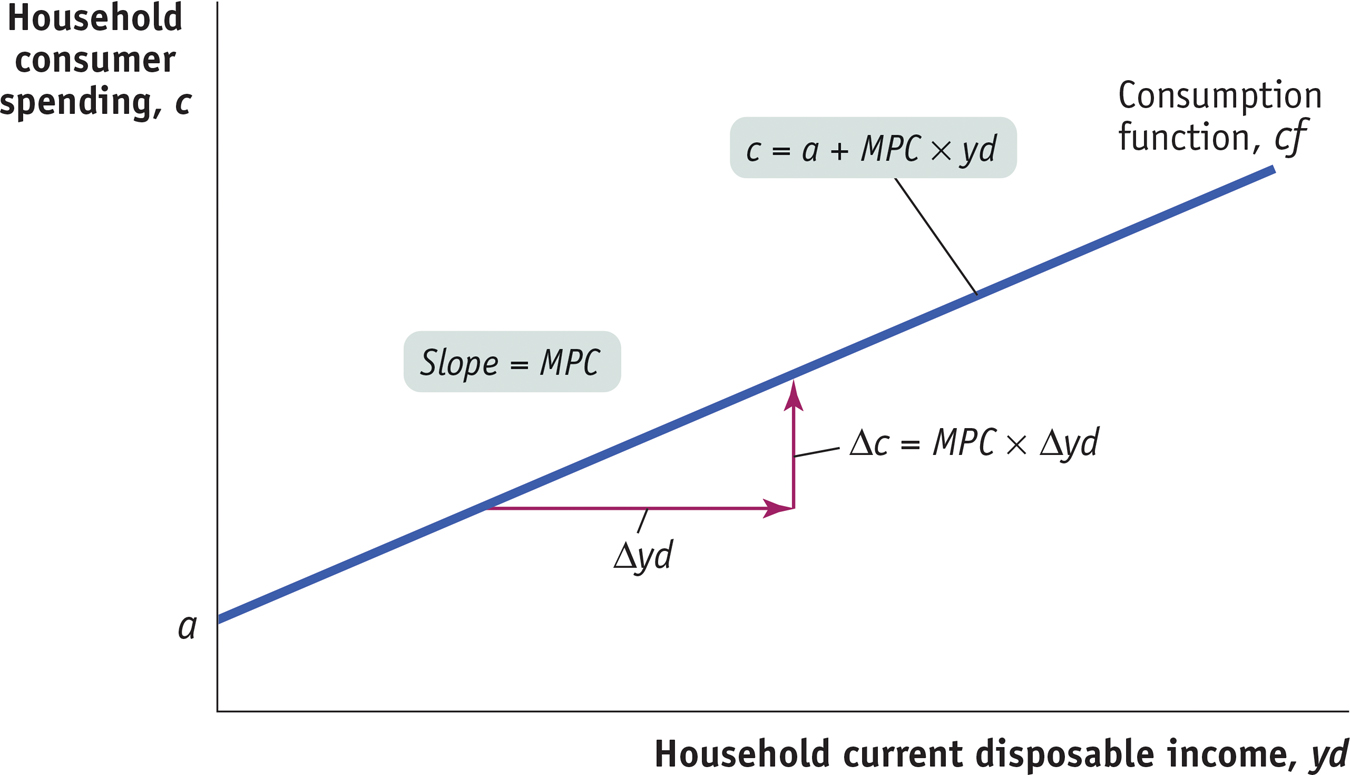
The Consumption Function The consumption function relates a household’s current disposable income to its consumer spending. The vertical intercept, a, is individual household autonomous consumer spending: the amount of a household’s consumer spending if its current disposable income is zero. The slope of the consumption function line, cf, is the marginal propensity to consume, or MPC: of every additional $1 of current disposable income, MPC × $1 is spent.
In reality, actual data never fit Equation 11-5 perfectly, but the fit can be pretty good. Figure 11-4 shows the data from Figure 11-2 again, together with a line drawn to fit the data as closely as possible. According to the data on households’ consumer spending and current disposable income, the best estimate of a is $19,343 and of MPC is 0.50. So the consumption function fitted to the data is:
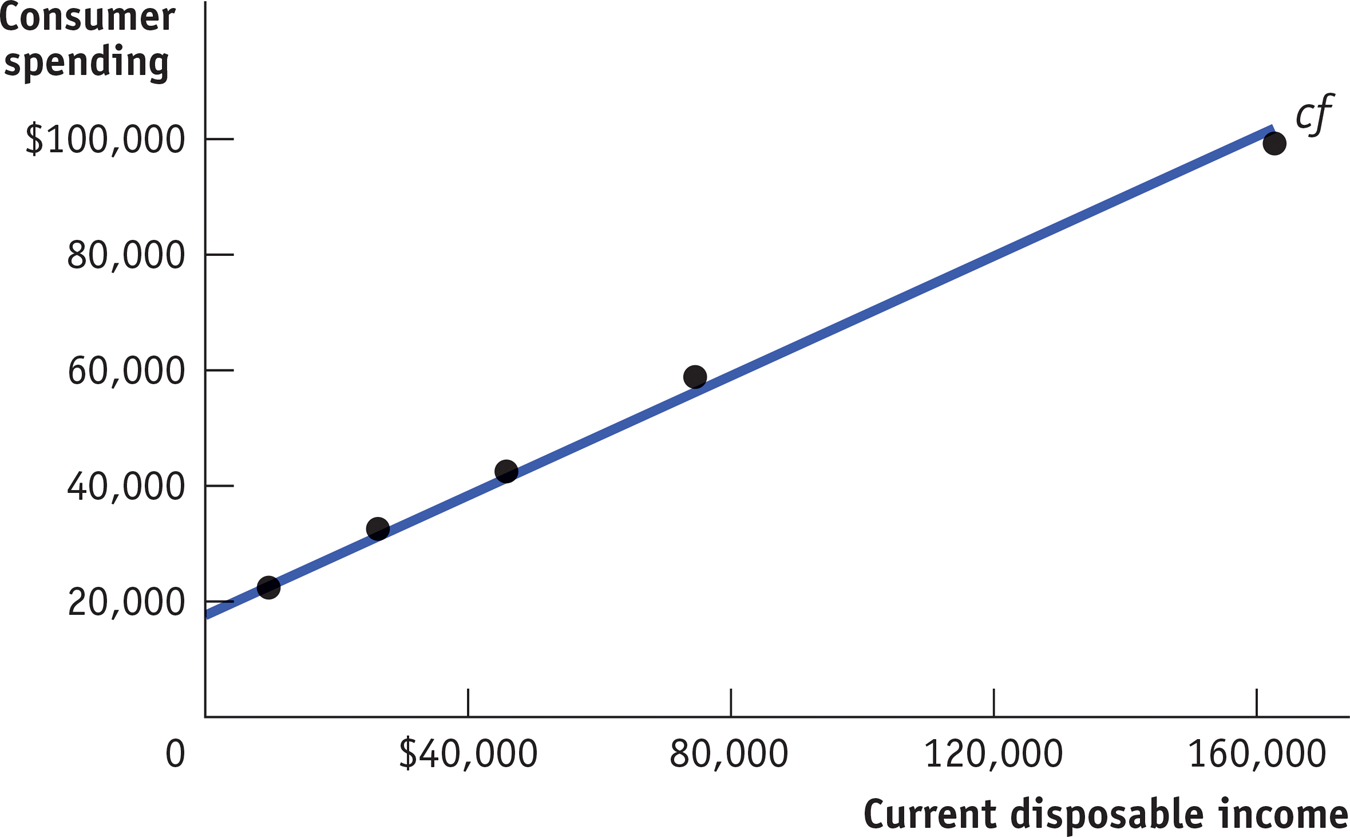
A Consumption Function Fitted to Data The data from Figure 11-2 are reproduced here, along with a line drawn to fit the data as closely as possible. For American households in 2013, the best estimate of the average household’s autonomous consumer spending, a, is $19,343 and the best estimate of MPC is 0.50. Source: Bureau of Labor Statistics.
That is, the data suggest a marginal propensity to consume of approximately 0.50. This implies that the marginal propensity to save (MPS)—the amount of an additional $1 of disposable income that is saved—is approximately 0.50, and the multiplier is approximately 1/0.50 = 2.00.
It’s important to realize that Figure 11-4 shows a microeconomic relationship between the current disposable income of individual households and their spending on goods and services. However, macroeconomists assume that a similar relationship holds for the economy as a whole: that there is a relationship, called the aggregate consumption function, between aggregate current disposable income and aggregate consumer spending. We’ll assume that it has the same form as the household-level consumption function:
The aggregate consumption function is the relationship for the economy as a whole between aggregate current disposable income and aggregate consumer spending.
Here, C is aggregate consumer spending (called just “consumer spending”); YD is aggregate current disposable income (called, for simplicity, just “disposable income”); and A is aggregate autonomous consumer spending, the amount of consumer spending when YD equals zero. This is the relationship represented in Figure 11-5 by CF, analogous to cf in Figure 11-3.
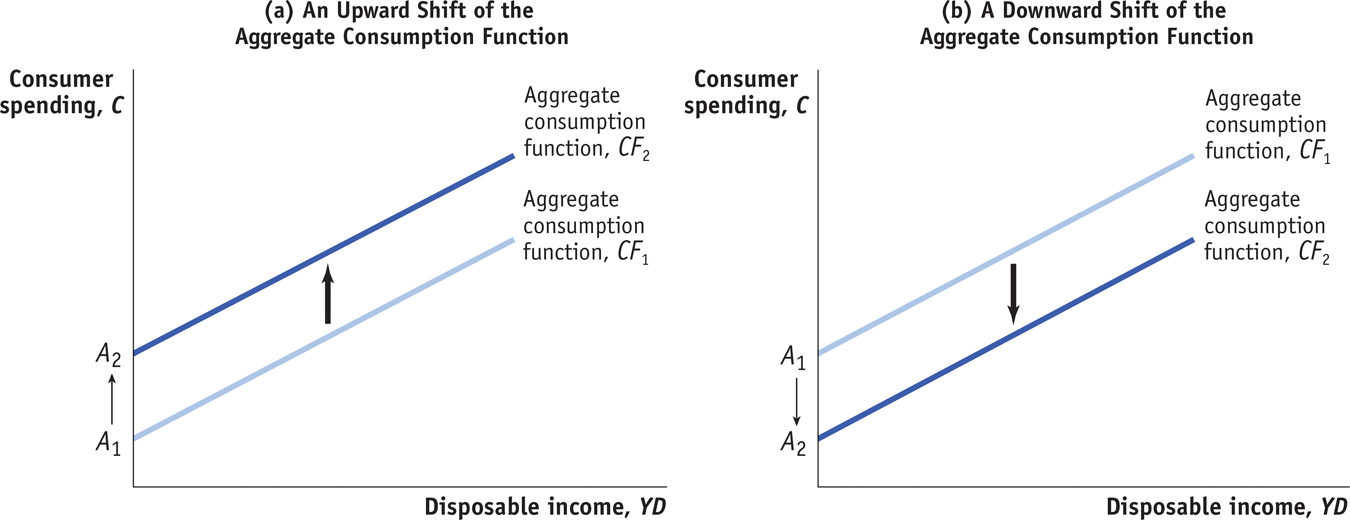
Shifts of the Aggregate Consumption Function Panel (a) illustrates the effect of an increase in expected aggregate future disposable income. Consumers will spend more at every given level of aggregate current disposable income, YD. As a result, the initial aggregate consumption function CF1, with aggregate autonomous consumer spending A1, shifts up to a new position at CF2 and aggregate autonomous consumer spending A2. An increase in aggregate wealth will also shift the aggregate consumption function up. Panel (b), in contrast, illustrates the effect of a reduction in expected aggregate future disposable income. Consumers will spend less at every given level of aggregate current disposable income, YD. Consequently, the initial aggregate consumption function CF1, with aggregate autonomous consumer spending A1, shifts down to a new position at CF2 and aggregate autonomous consumer spending A2. A reduction in aggregate wealth will have the same effect.