Short-Run Macroeconomic Equilibrium
We’ll begin our analysis by focusing on the short run. Figure 12-11 shows the aggregate demand curve and the short-run aggregate supply curve on the same diagram. The point at which the AD and SRAS curves intersect, ESR, is the short-run macroeconomic equilibrium: the point at which the quantity of aggregate output supplied is equal to the quantity demanded by domestic households, businesses, the government, and the rest of the world. The aggregate price level at ESR, PE, is the short-run equilibrium aggregate price level. The level of aggregate output at ESR, YE, is the short-run equilibrium aggregate output.
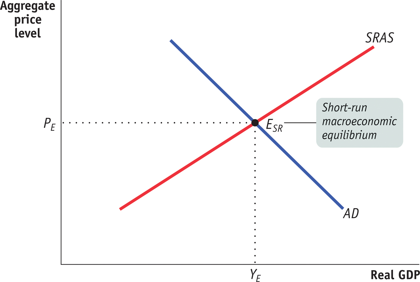
The AD–AS Model The AD–AS model combines the aggregate demand curve and the short-run aggregate supply curve. Their point of intersection, ESR, is the point of short-run macroeconomic equilibrium where the quantity of aggregate output demanded is equal to the quantity of aggregate output supplied. PE is the short-run equilibrium aggregate price level, and YE is the short-run equilibrium level of aggregate output.
The economy is in short-run macroeconomic equilibrium when the quantity of aggregate output supplied is equal to the quantity demanded.
The short-run equilibrium aggregate price level is the aggregate price level in the short-run macroeconomic equilibrium.
Short-run equilibrium aggregate output is the quantity of aggregate output produced in the short-run macroeconomic equilibrium.
In the supply and demand model of Chapter 3 we saw that a shortage of any individual good causes its market price to rise but a surplus of the good causes its market price to fall. These forces ensure that the market reaches equilibrium. The same logic applies to short-run macroeconomic equilibrium. If the aggregate price level is above its equilibrium level, the quantity of aggregate output supplied exceeds the quantity of aggregate output demanded. This leads to a fall in the aggregate price level and pushes it toward its equilibrium level.
If the aggregate price level is below its equilibrium level, the quantity of aggregate output supplied is less than the quantity of aggregate output demanded. This leads to a rise in the aggregate price level, again pushing it toward its equilibrium level. In the discussion that follows, we’ll assume that the economy is always in short-run macroeconomic equilibrium.
We’ll also make another important simplification based on the observation that in reality there is a long-term upward trend in both aggregate output and the aggregate price level. We’ll assume that a fall in either variable really means a fall compared to the long-run trend. For example, if the aggregate price level normally rises 4% per year, a year in which the aggregate price level rises only 3% would count, for our purposes, as a 1% decline. In fact, since the Great Depression there have been very few years in which the aggregate price level of any major nation actually declined—Japan’s period of deflation since 1995 is one of the few exceptions. We’ll explain why in Chapter 16. There have, however, been many cases in which the aggregate price level fell relative to the long-run trend.
Short-run equilibrium aggregate output and the short-run equilibrium aggregate price level can change either because of shifts of the AD curve or because of shifts of the SRAS curve. Let’s look at each case in turn.