Shifts of the Aggregate Demand Curve
In Chapter 3, where we introduced the analysis of supply and demand in the market for an individual good, we stressed the importance of the distinction between movements along the demand curve and shifts of the demand curve. The same distinction applies to the aggregate demand curve. Figure 12-1 shows a movement along the aggregate demand curve, a change in the aggregate quantity of goods and services demanded as the aggregate price level changes.
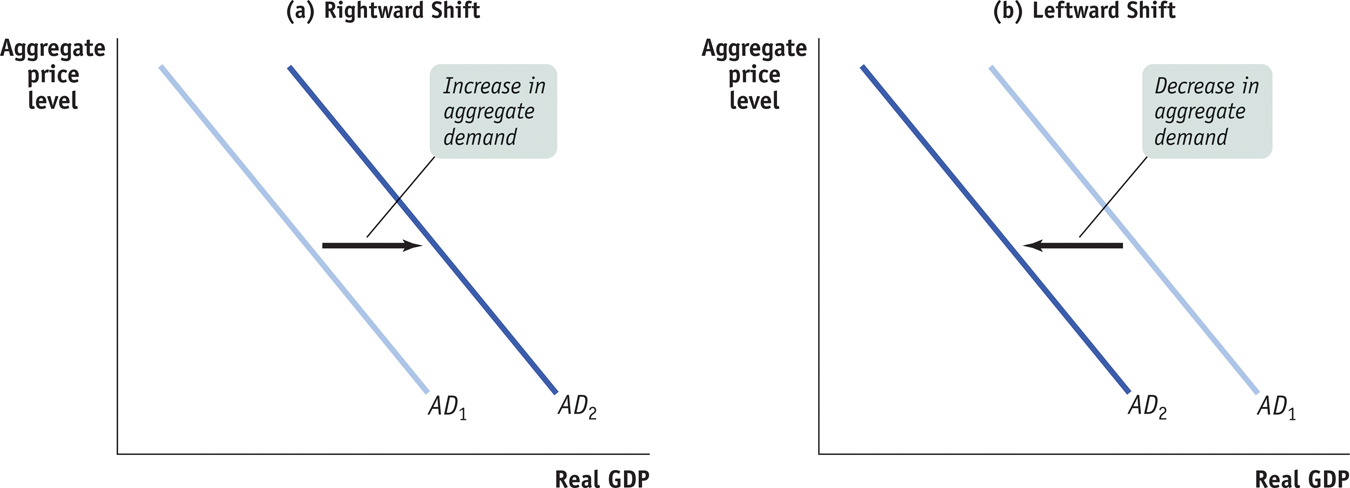
But there can also be shifts of the aggregate demand curve, changes in the quantity of goods and services demanded at any given price level, as shown in Figure 12-4. When we talk about an increase in aggregate demand, we mean a shift of the aggregate demand curve to the right, as shown in panel (a) by the shift from AD1 to AD2. A rightward shift occurs when the quantity of aggregate output demanded increases at any given aggregate price level. A decrease in aggregate demand means that the AD curve shifts to the left, as in panel (b). A leftward shift implies that the quantity of aggregate output demanded falls at any given aggregate price level.
A number of factors can shift the aggregate demand curve. Among the most important factors are changes in expectations, changes in wealth, and the size of the existing stock of physical capital. In addition, both fiscal and monetary policy can shift the aggregate demand curve. All five factors set the multiplier process in motion. By causing an initial rise or fall in real GDP, they change disposable income, which leads to additional changes in aggregate spending, which lead to further changes in real GDP, and so on. For an overview of factors that shift the aggregate demand curve, see Table 12-1 below.
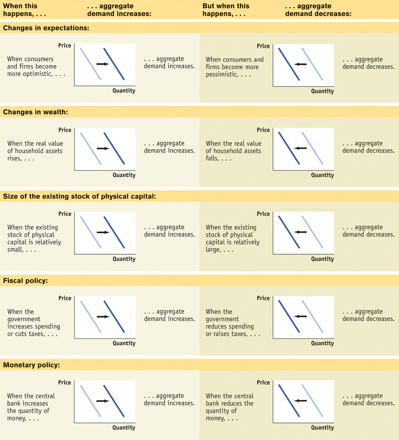
Changes in Expectations As explained in Chapter 11, both consumer spending and planned investment spending depend in part on people’s expectations about the future. Consumers base their spending not only on the income they have now but also on the income they expect to have in the future. Firms base their planned investment spending not only on current conditions but also on the sales they expect to make in the future. As a result, changes in expectations can push consumer spending and planned investment spending up or down. If consumers and firms become more optimistic, aggregate spending rises; if they become more pessimistic, aggregate spending falls.
In fact, short-
PITFALLS: CHANGES IN WEALTH: A MOVEMENT ALONG VERSUS A SHIFT OF THE AGGREGATE DEMAND CURVE
CHANGES IN WEALTH: A MOVEMENT ALONG VERSUS A SHIFT OF THE AGGREGATE DEMAND CURVE
Earlier we explained that one reason the AD curve is downward sloping is the wealth effect of a change in the aggregate price level: a higher aggregate price level reduces the purchasing power of households’ assets and leads to a fall in consumer spending, C. But we’ve just explained that changes in wealth lead to a shift of the AD curve. Aren’t those two explanations contradictory? Which one is it—
For example, a fall in the aggregate price level increases the purchasing power of consumers’ assets and leads to a movement down the AD curve. In contrast, a change in wealth independent of a change in the aggregate price level shifts the AD curve. For example, a rise in the stock market or a rise in real estate values leads to an increase in the real value of consumers’ assets at any given aggregate price level. In this case, the source of the change in wealth is a change in the values of assets without any change in the aggregate price level—
Changes in Wealth Consumer spending depends in part on the value of household assets. When the real value of these assets rises, the purchasing power they embody also rises, leading to an increase in aggregate spending. For example, in the 1990s there was a significant rise in the stock market that increased aggregate demand. And when the real value of household assets falls—

Size of the Existing Stock of Physical Capital Firms engage in planned investment spending to add to their stock of physical capital. Their incentive to spend depends in part on how much physical capital they already have: the more they have, the less they will feel a need to add more, other things equal. The same applies to other types of investment spending—