The Equilibrium Interest Rate
Recall that, for simplicity, we’re assuming there is only one interest rate paid on nonmonetary financial assets, both in the short run and in the long run. To understand how the interest rate is determined, consider Figure 15-3, which illustrates the liquidity preference model of the interest rate; this model says that the interest rate is determined by the supply and demand for money in the market for money. Figure 15-3 combines the money demand curve, MD, with the money supply curve, MS, which shows how the quantity of money supplied by the Federal Reserve varies with the interest rate.
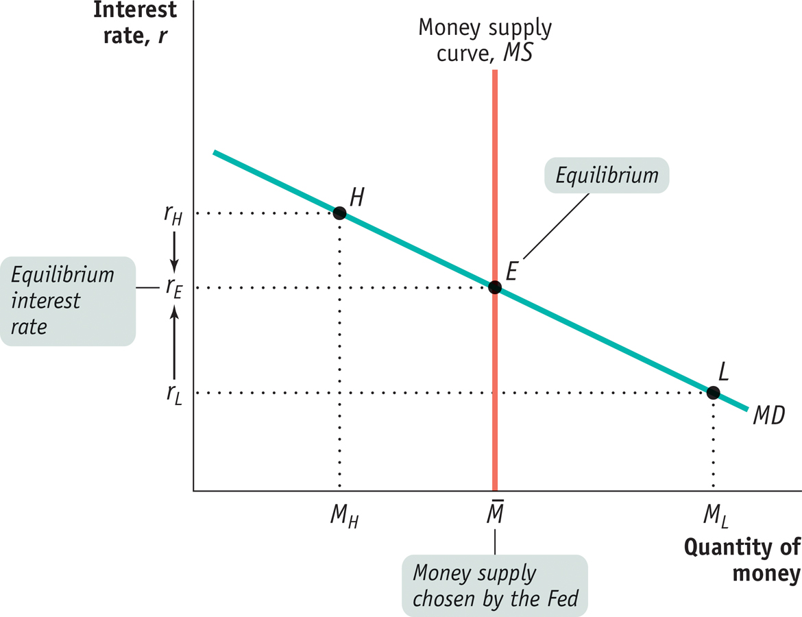
 . The money market is in equilibrium at the interest rate rE: the quantity of money demanded by the public is equal to , the quantity of money supplied.
At a point such as L, the interest rate, rL, is below rE and the corresponding quantity of money demanded, ML, exceeds the money supply,
. In an attempt to shift their wealth out of nonmoney interest-. In an attempt to shift out of money holdings into nonmoney interest-According to the liquidity preference model of the interest rate, the interest rate is determined by the supply and demand for money.
The money supply curve shows how the quantity of money supplied varies with the interest rate.
In Chapter 14 we learned how the Federal Reserve can increase or decrease the money supply: it usually does this through open-. The money market equilibrium is at E, where MS and MD cross. At this point the quantity of money demanded equals the money supply, , leading to an equilibrium interest rate of rE.
To understand why rE is the equilibrium interest rate, consider what happens if the money market is at a point like L, where the interest rate, rL, is below rE. At rL the public wants to hold the quantity of money ML, an amount larger than the actual money supply, . This means that at point L, the public wants to shift some of its wealth out of interest-
This result has two implications. One is that the quantity of money demanded is more than the quantity of money supplied. The other is that the quantity of interest-. That is, the interest rate will rise until it is equal to rE.
Now consider what happens if the money market is at a point such as H in Figure 15-3, where the interest rate rH is above rE. In that case the quantity of money demanded, MH, is less than the quantity of money supplied, . Correspondingly, the quantity of interest-. Again, the interest rate will end up at rE.