Productivity is higher, other things equal, when workers are equipped with more physical capital, more human capital, better technology, or any combination of the three. But can we put numbers to these effects? To do this, economists make use of estimates of the aggregate production function, which shows how productivity depends on the quantities of physical capital per worker and human capital per worker as well as the state of technology.

In general, all three factors tend to rise over time, as workers are equipped with more machinery, receive more education, and benefit from technological advances. What the aggregate production function does is allow economists to disentangle the effects of these three factors on overall productivity.

An example of an aggregate production function applied to real data comes from a comparative study of Chinese and Indian economic growth by the economists Barry Bosworth and Susan Collins of the Brookings Institution. They used the following aggregate production function:

where T represented an estimate of the level of technology and they assumed that each year of education raises workers’ human capital by 7%. Using this function, they tried to explain why China grew faster than India between 1978 and 2004. About half the difference, they found, was due to China’s higher levels of investment spending, which raised its level of physical capital per worker faster than India’s. The other half was due to faster Chinese technological progress.

In analyzing historical economic growth, economists have discovered a crucial fact about the estimated aggregate production function: it exhibits diminishing returns to physical capital. That is, when the amount of human capital per worker and the state of technology are held fixed, each successive increase in the amount of physical capital per worker leads to a smaller increase in productivity.

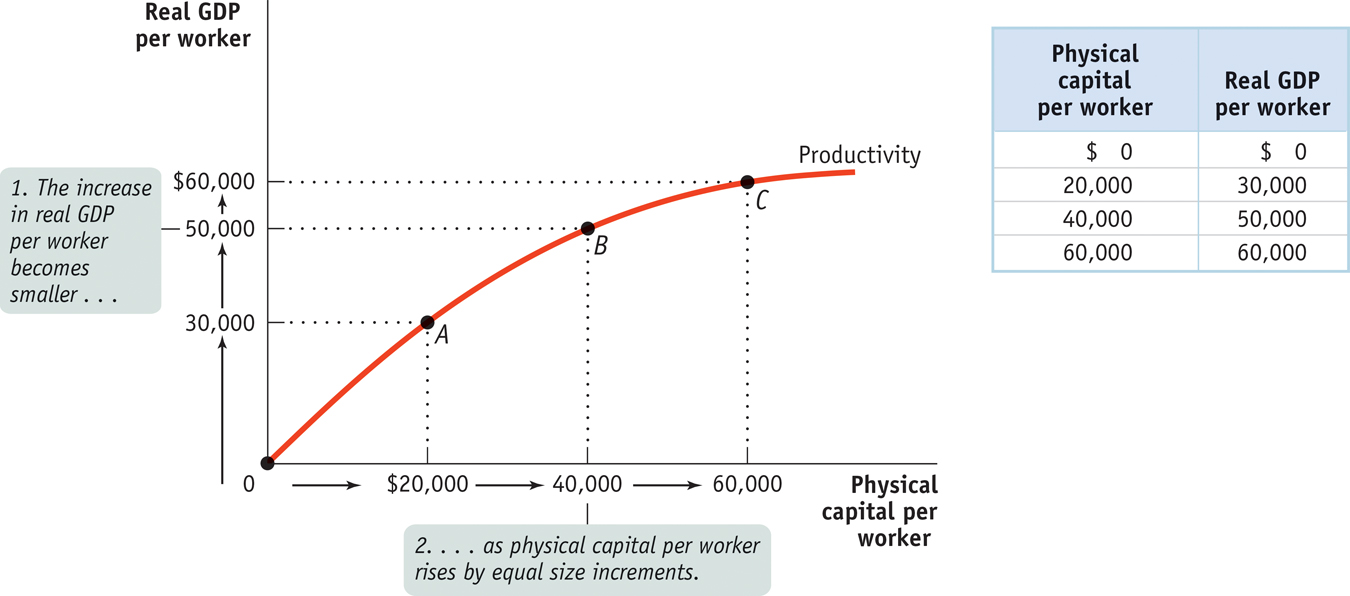
Figure 9-4 and the table to its right give a hypothetical example of how the level of physical capital per worker might affect the level of real GDP per worker, holding human capital per worker and the state of technology fixed. In this example, we measure the quantity of physical capital in dollars.

To see why the relationship between physical capital per worker and productivity exhibits diminishing returns, think about how having farm equipment affects the productivity of farmworkers. A little bit of equipment makes a big difference: a worker equipped with a tractor can do much more than a worker without one. And a worker using more expensive equipment will, other things equal, be more productive: a worker with a $40,000 tractor will normally be able to cultivate more farmland in a given amount of time than a worker with a $20,000 tractor because the more expensive machine will be more powerful, perform more tasks, or both.

But will a worker with a $40,000 tractor, holding human capital and technology constant, be twice as productive as a worker with a $20,000 tractor? Probably not: there’s a huge difference between not having a tractor at all and having even an inexpensive tractor; there’s much less difference between having an inexpensive tractor and having a better tractor. And we can be sure that a worker with a $200,000 tractor won’t be 10 times as productive: a tractor can be improved only so much. Because the same is true of other kinds of equipment, the aggregate production function shows diminishing returns to physical capital.

Diminishing returns to physical capital imply a relationship between physical capital per worker and output per worker like the one shown in Figure 9-4. As the productivity curve for physical capital and the accompanying table illustrate, more physical capital per worker leads to more output per worker. But each $20,000 increment in physical capital per worker adds less to productivity.

As you can see from the table, there is a big payoff for the first $20,000 of physical capital: real GDP per worker rises by $30,000. The second $20,000 of physical capital also raises productivity, but not by as much: real GDP per worker goes up by only $20,000. The third $20,000 of physical capital raises real GDP per worker by only $10,000. By comparing points along the curve you can also see that as physical capital per worker rises, output per worker also rises—but at a diminishing rate. Going from the origin at 0 to point A, a $20,000 increase in physical capital per worker, leads to an increase of $30,000 in real GDP per worker. Going from point A to point B, a second $20,000 increase in physical capital per worker, leads to an increase of only $20,000 in real GDP per worker. And from point B to point C, a $20,000 increase in physical capital per worker, increased real GDP per worker by only $10,000.

It’s important to realize that diminishing returns to physical capital is an “other things equal” phenomenon: additional amounts of physical capital are less productive when the amount of human capital per worker and the technology are held fixed. Diminishing returns may disappear if we increase the amount of human capital per worker, or improve the technology, or both at the same time the amount of physical capital per worker is increased.

For example, a worker with a $40,000 tractor who has also been trained in the most advanced cultivation techniques may in fact be more than twice as productive as a worker with only a $20,000 tractor and no additional human capital. But diminishing returns to any one input—regardless of whether it is physical capital, human capital, or number of workers—is a pervasive characteristic of production. Typical estimates suggest that in practice a 1% increase in the quantity of physical capital per worker increases output per worker by only one-third of 1%, or 0.33%.

In practice, all the factors contributing to higher productivity rise during the course of economic growth: both physical capital and human capital per worker increase, and technology advances as well. To disentangle the effects of these factors, economists use growth accounting, which estimates the contribution of each major factor in the aggregate production function to economic growth. For example, suppose the following are true:

In that case, we would estimate that growing physical capital per worker is responsible for 3% × 0.33 = 1 percentage point of productivity growth per year. A similar but more complex procedure is used to estimate the effects of growing human capital. The procedure is more complex because there aren’t simple dollar measures of the quantity of human capital.

Growth accounting allows us to calculate the effects of greater physical and human capital on economic growth. But how can we estimate the effects of technological progress? We do so by estimating what is left over after the effects of physical and human capital have been taken into account. For example, let’s imagine that there was no increase in human capital per worker so that we can focus on changes in physical capital and in technology.

In Figure 9-5, the lower curve shows the same hypothetical relationship between physical capital per worker and output per worker shown in Figure 9-4. Let’s assume that this was the relationship given the technology available in 1940. The upper curve also shows a relationship between physical capital per worker and productivity, but this time given the technology available in 2010. (We’ve chosen a 70-year stretch to allow us to use the Rule of 70.) The 2010 curve is shifted up compared to the 1940 curve because technologies developed over the previous 70 years make it possible to produce more output for a given amount of physical capital per worker than was possible with the technology available in 1940. (Note that the two curves are measured in constant dollars.)

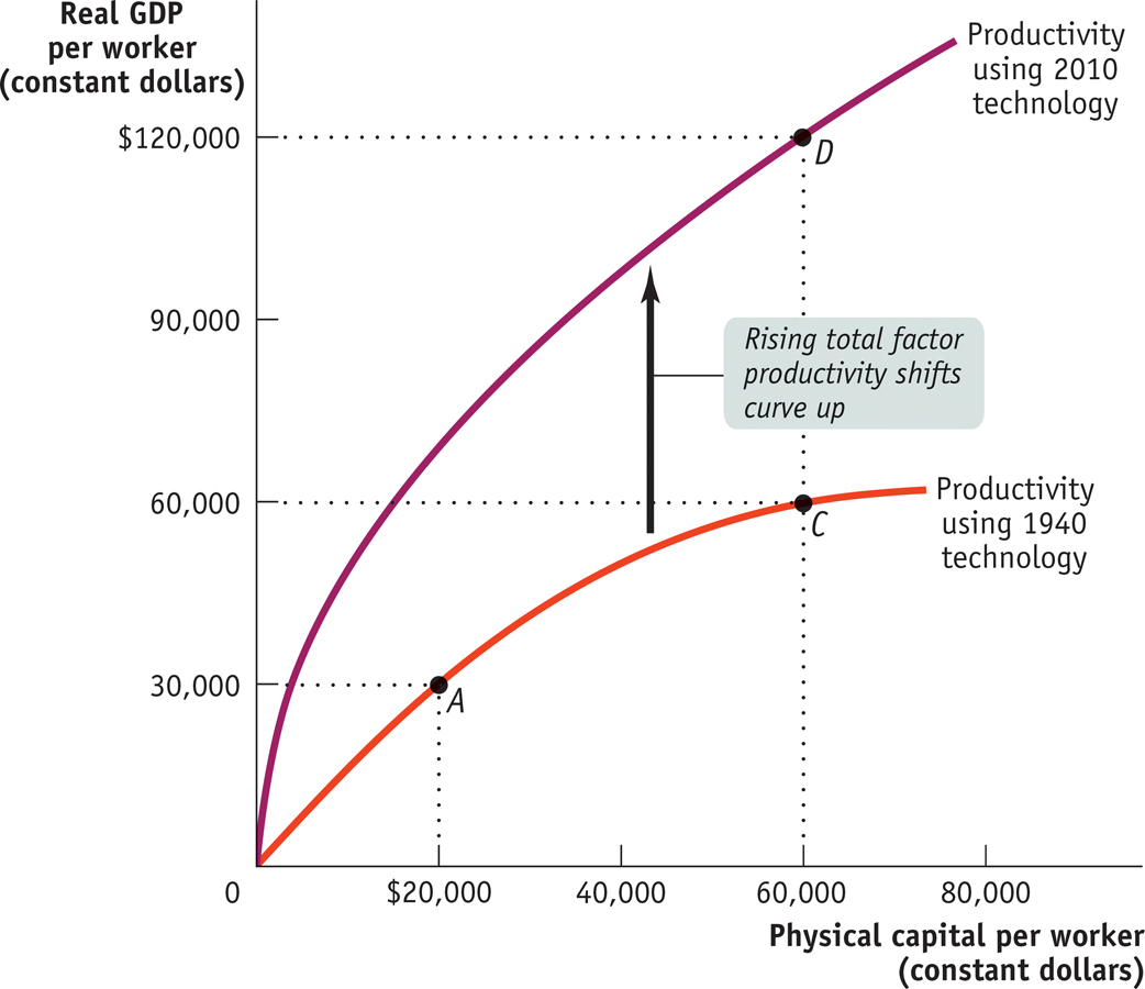
Let’s assume that between 1940 and 2010 the amount of physical capital per worker rose from $20,000 to $60,000. If this increase in physical capital per worker had taken place without any technological progress, the economy would have moved from A to C: output per worker would have risen, but only from $30,000 to $60,000, or 1% per year (using the Rule of 70 tells us that a 1% growth rate over 70 years doubles output). In fact, however, the economy moved from A to D: output rose from $30,000 to $120,000, or 2% per year. There was an increase in both physical capital per worker and technological progress, which shifted the aggregate production function.

In this case, 50% of the annual 2% increase in productivity—that is, 1% in annual productivity growth—is due to higher total factor productivity, the amount of output that can be produced with a given amount of factor inputs. So when total factor productivity increases, the economy can produce more output with the same quantity of physical capital, human capital, and labor.

Most estimates find that increases in total factor productivity are central to a country’s economic growth. We believe that observed increases in total factor productivity in fact measure the economic effects of technological progress. All of this implies that technological change is crucial to economic growth.

The Bureau of Labor Statistics estimates the growth rate of both labor productivity and total factor productivity for nonfarm business in the United States. According to the Bureau’s estimates, over the period from 1948 to 2010 American labor productivity rose 2.3% per year. Only 49% of that rise is explained by increases in physical and human capital per worker; the rest is explained by rising total factor productivity—that is, by technological progress.