1.4 Module 34: Monopolistic Competition

iStockphoto

Understanding Monopolistic Competition

Suppose an industry is monopolistically competitive: it consists of many producers, all competing for the same consumers but offering differentiated products. There is also free entry into and exit from the industry in the long run. How does such an industry behave?

As the term monopolistic competition suggests, this market structure combines some features typical of monopoly with others typical of perfect competition. Because each firm is offering a distinct product, it is in a way like a monopolist: it faces a downward-sloping demand curve and has some market power—the ability within limits to determine the price of its product.

However, unlike a pure monopolist, a monopolistically competitive firm does face competition: the amount of its product it can sell depends on the prices and products offered by other firms in the industry.

The same, of course, is true of an oligopoly. In a monopolistically competitive industry, however, there are many producers, as opposed to the small number that defines an oligopoly. This means that the “puzzle” of oligopoly—whether firms will collude or behave noncooperatively—does not arise in the case of monopolistically competitive industries. True, if all the gas stations or all the restaurants in a town could agree—explicitly or tacitly—to raise prices, it would be in their mutual interest to do so. But such collusion is virtually impossible when the number of firms is large and, by implication, there are no barriers to entry.

So in situations of monopolistic competition, we can safely assume that firms behave noncooperatively and ignore the potential for collusion.

Monopolistic Competition in the Short Run

We introduced the distinction between short-run and long-run equilibrium when we studied perfect competition. The short-run equilibrium of an industry takes the number of firms as given. The long-run equilibrium, by contrast, is reached only after enough time has elapsed for firms to enter or exit the industry. To analyze monopolistic competition, we focus first on the short run and then on how an industry moves from the short run to the long run.

Panels (a) and (b) of Figure 34-1 show two possible situations that a typical firm in a monopolistically competitive industry might face in the short run. In each case, the firm looks like any monopolist: it faces a downward-sloping demand curve, which implies a downward-sloping marginal revenue curve.

The firm in panel (a) can be profitable for some output quantities: the quantities for which its average total cost curve, ATC, lies below its demand curve, D_P. The profitmaximizing output quantity is Q_P, the output at which marginal revenue, MR_P, is equal to marginal cost, MC. The firm charges price P_P and earns a profit, represented by the area of the green shaded rectangle. The firm in panel (b), however, can never be profitable because its average total cost curve lies above its demand curve, D_U, for every output quantity. The best that it can do if it produces at all is to produce quantity Q_U and charge price P_U. This generates a loss, indicated by the area of the yellow shaded rectangle. Any other output quantity results in a greater loss.

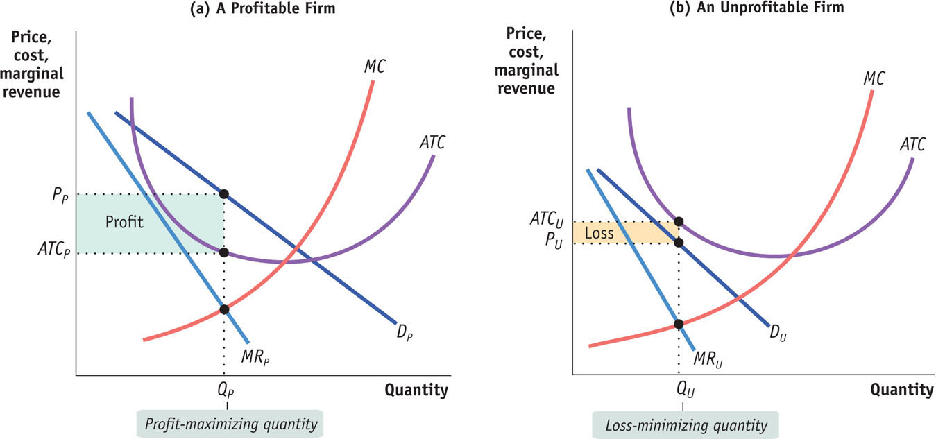
We assume that every firm has an upward-sloping marginal cost curve but that it also faces some fixed costs, so that its average total cost curve is U-shaped. This assumption doesn’t matter in the short run; but, as we’ll see shortly, it is crucial to understanding the long-run equilibrium.

In each case the firm, in order to maximize profit, sets marginal revenue equal to marginal cost. So how do these two figures differ? In panel (a) the firm is profitable; in panel (b) it is unprofitable. (Recall that we are referring always to economic profit and not accounting profit—that is, a profit given that all factors of production are earning their opportunity costs.)

In panel (a) the firm faces the demand curve D_P and the marginal revenue curve MR_P. It produces the profit-maximizing output Q_P, the quantity at which marginal revenue is equal to marginal cost, and sells it at the price P_P. This price is above the average total cost at this output, ATC_P. The firm’s profit is indicated by the area of the shaded rectangle.

In panel (b) the firm faces the demand curve D_U and the marginal revenue curve MR_U. It chooses the quantity Q_U at which marginal revenue is equal to marginal cost. However, in this case the price P_U is below the average total cost ATC_U; so at this quantity the firm loses money. Its loss is equal to the area of the shaded rectangle. Since Q_U is the profit-maximizing quantity—which means, in this case, the loss-minimizing quantity—there is no way for a firm in this situation to make a profit. We can confirm this by noting that at any quantity of output, the average total cost curve in panel (b) lies above the demand curve D_U. Because ATC > P at all quantities of output, this firm always suffers a loss.

As this comparison suggests, the key to whether a firm with market power is profitable or unprofitable in the short run lies in the relationship between its demand curve and its average total cost curve. In panel (a) the demand curve D_P crosses the average total cost curve, meaning that some of the demand curve lies above the average total cost curve. So there are some price–quantity combinations available at which price is higher than average total cost, indicating that the firm can choose a quantity at which it makes positive profit.

In panel (b), by contrast, the demand curve D_U does not cross the average total cost curve—it always lies below it. So the price corresponding to each quantity demanded is always less than the average total cost of producing that quantity. There is no quantity at which the firm can avoid losing money.

These figures, showing firms facing downward-sloping demand curves and their associated marginal revenue curves, look just like ordinary monopoly graphs. The “competition” aspect of monopolistic competition comes into play, however, when we move from the short run to the long run.

Monopolistic Competition in the Long Run

Obviously, an industry in which existing firms are losing money, like the one in panel (b) of Figure 34-1, is not in long-run equilibrium. When existing firms are losing money, some firms will exit the industry. The industry will not be in long-run equilibrium until the persistent losses have been eliminated by the exit of some firms.

In the long run, profit lures new firms to enter an industry.

© Brooke Becker/Dreamstime.com

It may be less obvious that an industry in which existing firms are earning profits, like the one in panel (a) of Figure 34-1, is also not in long-run equilibrium. Given there is free entry into the industry, persistent profits earned by the existing firms will lead to the entry of additional producers. The industry will not be in long-run equilibrium until the persistent profits have been eliminated by the entry of new producers.

How will entry or exit by other firms affect the profit of a typical existing firm? Because the differentiated products offered by firms in a monopolistically competitive industry are available to the same set of customers, entry or exit by other firms will affect the demand curve facing every existing producer.

If new gas stations open along a highway, each of the existing gas stations will no longer be able to sell as much gas as before at any given price. So, as illustrated in panel (a) of Figure 34-2, entry of additional producers into a monopolistically competitive industry will lead to a leftward shift of the demand curve and the marginal revenue curve facing a typical existing producer.

Entry will occur in the long run when existing firms are profitable. In panel (a), entry causes each existing firm’s demand curve and marginal revenue curve to shift to the left. The firm receives a lower price for every unit it sells, and its profit falls. Entry will cease when firms make zero profit. Exit will occur in the long run when existing firms are unprofitable. In panel (b), exit from the industry shifts each remaining firm’s demand curve and marginal revenue curve to the right. The firm receives a higher price for every unit it sells, and profit rises. Exit will cease when the remaining firms make zero profit.

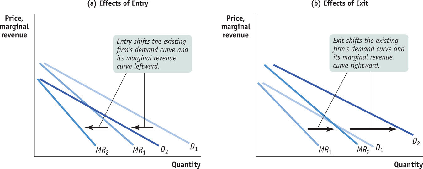
Conversely, suppose that some of the gas stations along the highway close. Then each of the remaining stations will be able to sell more gasoline at any given price. So as illustrated in panel (b), exit of firms from an industry leads to a rightward shift of the demand curve and marginal revenue curve facing a typical remaining producer.

The industry will be in long-run equilibrium when there is neither entry nor exit. This will occur only when every firm earns zero profit. So in the long run, a monopolistically competitive industry will end up in zero-profit equilibrium, in which firms just manage to cover their costs at their profit-maximizing output quantities.

We have seen that a firm facing a downward-sloping demand curve will earn positive profit if any part of that demand curve lies above its average total cost curve; it will incur a loss if its entire demand curve lies below its average total cost curve. So in zero-profit equilibrium, the firm must be in a borderline position between these two cases; its demand curve must just touch its average total cost curve. That is, the demand curve must be just tangent to the average total cost curve (meaning it just touches the curve) at the firm’s profit-maximizing output quantity—the output quantity at which marginal revenue equals marginal cost.

If this is not the case, the firm operating at its profit-maximizing quantity will find itself making either a profit or loss, as illustrated in the panels of Figure 34-1. But we also know that free entry and exit means that this cannot be a long-run equilibrium. Why?

In the case of a profit, new firms will enter the industry, shifting the demand curve of every existing firm leftward until all profit is eliminated. In the case of a loss, some existing firms exit and so shift the demand curve of every remaining firm to the right until all losses are eliminated. All entry and exit ceases only when every existing firm makes zero profit at its profit-maximizing quantity of output.

Figure 34-3 shows a typical monopolistically competitive firm in such a zero-profit equilibrium. The firm produces Q_MC, the output at which MR_MC = MC, and charges price P_MC. At this price and quantity, represented by point Z, the demand curve is just tangent to its average total cost curve. The firm earns zero profit because price, P_MC, is equal to average total cost, ATC_MC.

If existing firms are profitable, entry will occur and shift each existing firm’s demand curve leftward. If existing firms are unprofitable, each remaining firm’s demand curve shifts rightward as some firms exit the industry. Entry and exit will cease when every existing firm makes zero profit at its profit-maximizing quantity. So, in long-run zero-profit equilibrium, the demand curve of each firm is tangent to its average total cost curve at its profit-maximizing quantity: at the profit-maximizing quantity, Q_MC, price, P_MC, equals average total cost, ATC_MC. A monopolistically competitive firm is like a monopolist without monopoly profits.

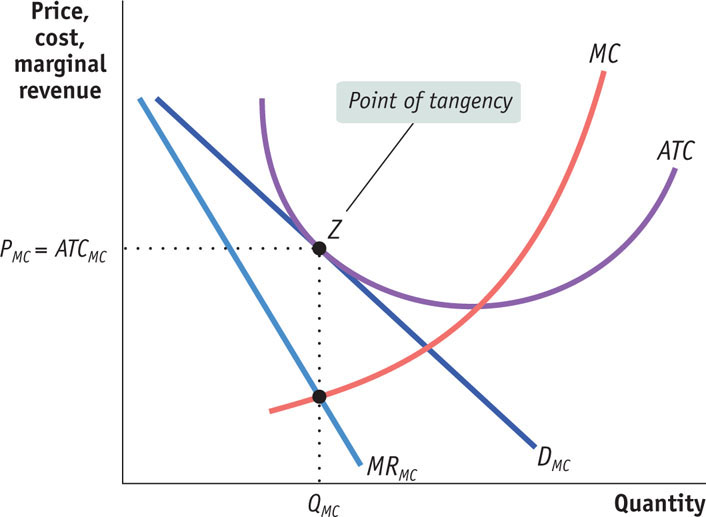
The normal long-run condition of a monopolistically competitive industry, then, is that each producer is in the situation shown in Figure 34-3. Each producer acts like a monopolist, facing a downward-sloping demand curve and setting marginal cost equal to marginal revenue so as to maximize profit. But this is just enough to achieve zero economic profit. The producers in the industry are like monopolists without monopoly profit.

THE HOUSING BUST AND THE DEMISE OF THE 6% COMMISSION

The vast majority of home sales in the United States are transacted with the use of real estate agents. A home-owner looking to sell hires an agent, who lists the house for sale and shows it to interested buyers. Correspondingly, prospective home buyers hire their own agent to arrange inspections of available houses.

Traditionally, agents were paid by the seller: a commission equal to 6% of the sales price of the house, which the seller’s agent and the buyer’s agent would split equally. If a house sold for $300,000, for example, the seller’s agent and the buyer’s agent each received $9,000 (equal to 3% of $300,000).

The real estate brokerage industry fits the model of monopolistic competition quite well: in any given local market, there are many real estate agents, all competing with one another, but the agents are differentiated by location and personality as well as by the type of home they sell (whether condominiums, very expensive homes, and so on). And the industry has free entry: it’s relatively easy for someone to become a real estate agent (take a course and then pass a test to obtain a license).

Shutterstock

But for a long time there was one feature that didn’t fit the model of monopolistic competition: the fixed 6% commission that had not changed over time and was unaffected by the ups and downs of the housing market.

You may wonder how agents were able to maintain the 6% commission. Why didn’t new agents enter the market and drive the commission down to the zero-profit level? One tactic used by agents was their control of the Multiple Listing Service, or MLS, which lists nearly all the homes for sale in a community. Traditionally, only sellers who agreed to the 6% commission were allowed to list their homes on the MLS.

But protecting the 6% commission was always an iffy endeavor because any action by the brokerage industry to fix the commission rate at a given percentage would run afoul of antitrust laws. And by the early to mid-2000s, as the housing boom intensified, discount brokers had appeared on the scene. But traditional agents refused to work with them. So in 2005, the Justice Department sued the National Association of Realtors, the powerful trade group of agents.

In fact, oversight by regulators and the housing market bust which began in 2006 hastened the demise of the non-negotiable 6% commission. With sellers forced to accept less for their houses than often anticipated, agents were pressured to accept less as well. By 2009, the average commission fell to 5.36%, and agents were offering to list properties on broker databases for as little as a few hundred dollars. As Steve Murray, the editor of a trade publication, said in 2011, “The standard 6 percent went out the window a long time ago.”

Monopolistic Competition versus Perfect Competition

In a way, long-run equilibrium in a monopolistically competitive industry looks a lot like long-run equilibrium in a perfectly competitive industry. In both cases, there are many firms; in both cases, profits have been competed away; in both cases, the price received by every firm is equal to the average total cost of production.

However, the two versions of long-run equilibrium are different—in ways that are economically significant.

Price, Marginal Cost, and Average Total Cost

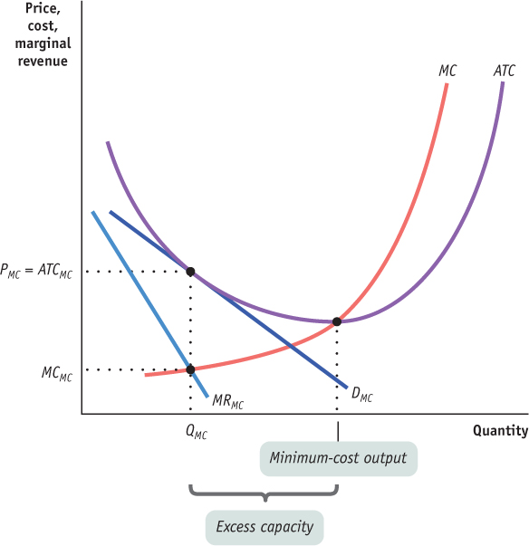
Figure 34-4 compares the long-run equilibrium of a typical firm in a perfectly competitive industry with that of a typical firm in a monopolistically competitive industry. Panel (a) shows a perfectly competitive firm facing a market price equal to its minimum average total cost; panel (b) reproduces Figure 34-3. Comparing the panels, we see two important differences.

First, in the case of the perfectly competitive firm shown in panel (a), the price, P_PC, received by the firm at the profit-maximizing quantity, Q_PC, is equal to the firm’s marginal cost of production, MC_PC, at that quantity of output. By contrast, at the profit-maximizing quantity chosen by the monopolistically competitive firm in panel (b), Q_MC, the price, P_MC, is higher than the marginal cost of production, MC_MC.

This difference translates into a difference in the attitude of firms toward consumers. A wheat farmer, who can sell as much wheat as he likes at the going market price, would not get particularly excited if you offered to buy some more wheat at the market price. Since he has no desire to produce more at that price and can sell the wheat to someone else, you are not doing him a favor.

But if you decide to fill up your tank at Jamil’s gas station rather than at Katy’s, you are doing Jamil a favor. He is not willing to cut his price to get more customers—he’s already made the best of that trade-off. But if he gets a few more customers than he expected at the posted price, that’s good news: an additional sale at the posted price increases his revenue more than it increases his cost because the posted price exceeds marginal cost.

The fact that monopolistic competitors, unlike perfect competitors, want to sell more at the going price is crucial to understanding why they engage in activities like advertising that help increase sales.

Panel (a) shows the situation of the typical firm in long-run equilibrium in a perfectly competitive industry. The firm operates at the minimum-cost output Q_PC, sells at the competitive market price P_PC, and makes zero profit. It is indifferent to selling another unit of output because P_PC is equal to its marginal cost, MC_PC. Panel (b) shows the situation of the typical firm in long-run equilibrium in a monopolistically competitive industry. At Q_MC it makes zero profit because its price, P_MC, just equals average total cost, ATC_MC. At Q_MC the firm would like to sell another unit at price P_MC since P_MC exceeds marginal cost, MC_MC. But it is unwilling to lower price to make more sales. It therefore operates to the left of the minimum-cost output level and has excess capacity.

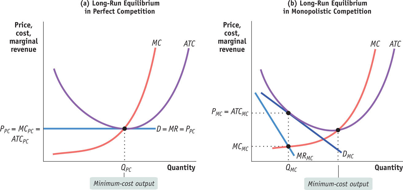
The other difference between monopolistic competition and perfect competition that is visible in Figure 34-4 involves the position of each firm on its average total cost curve. In panel (a), the perfectly competitive firm produces at point Q_PC, at the bottom of the U-shaped ATC curve. That is, each firm produces the quantity at which average total cost is minimized—the minimum-cost output. As a consequence, the total cost of industry output is also minimized.

Under monopolistic competition, in panel (b), the firm produces at Q_MC, on the downward-sloping part of the U-shaped ATC curve: it produces less than the quantity that would minimize average total cost. This failure to produce enough to minimize average total cost is sometimes described as the excess capacity issue. The typical vendor in a food court or a gas station along a road is not big enough to take maximum advantage of available cost savings. So the total cost of industry output is not minimized in the case of a monopolistically competitive industry.

Some people have argued that, because every monopolistic competitor has excess capacity, monopolistically competitive industries are inefficient. But the issue of efficiency under monopolistic competition turns out to be a subtle one that does not have a clear answer.

Is Monopolistic Competition Inefficient?

A monopolistic competitor, like a monopolist, charges a price that is above marginal cost. As a result, some people who are willing to pay at least as much for an egg roll at Wonderful Wok as it costs to produce it are deterred from doing so. In monopolistic competition, some mutually beneficial transactions go unexploited.

Furthermore, it is often argued that monopolistic competition is subject to a further kind of inefficiency: that the excess capacity of every monopolistic competitor implies wasteful duplication because monopolistically competitive industries offer too many varieties. According to this argument, it would be better if there were only two or three vendors in the food court, not six or seven. If there were fewer vendors, they would each have lower average total costs and so could offer food more cheaply.

Consumers benefit from the diversity of products offered in a monopolistically competitive industry.

iStockphoto

Is this argument against monopolistic competition right—that it lowers total surplus by causing inefficiency? Not necessarily. It’s true that if there were fewer gas stations along a highway, each gas station would sell more gasoline and so would have a lower cost per gallon. But there is a drawback: motorists would be inconvenienced because gas stations would be farther apart. The point is that the diversity of products offered in a monopolistically competitive industry is beneficial to consumers. So the higher price consumers pay because of excess capacity is offset to some extent by the value they receive from greater diversity.

There is, in other words, a trade-off: more producers mean higher average total costs but also greater product diversity. Does a monopolistically competitive industry arrive at the socially optimal point in this trade-off? Probably not—but it is hard to say whether there are too many firms or too few! Most economists now believe that duplication of effort and excess capacity in monopolistically competitive industries are not large problems in practice.

Module 34 Review

Check Your Understanding

Draw a correctly labeled graph for a monopolistically competitive firm in long-run equilibrium. Label the distance on the quantity axis that represents excess capacity.