1.3 42The Market for Labor

WHAT YOU WILL LEARN
 The way in which a worker’s decision about time preference gives rise to labor supply
 How to find equilibrium in the labor market
So far in this section we’ve focused on the demand for factors, which determines the quantities demanded of labor, capital, or land by producers as a function of their factor prices. But what about the supply of factors? In this module we focus exclusively on the supply of labor. Labor is the most important factor of production in the modern U.S. economy, accounting for most of factor income. We will look at how labor supply arises from a worker’s decision about time allocation and explore the determination of equilibrium wage and quantity in the labor market.
The Supply of Labor
There are only 24 hours in a day, so to supply labor is to give up leisure, which presents a dilemma of sorts. For this and other reasons, as we’ll see, the labor market looks different from markets for goods and services.
Work versus Leisure
In the labor market, the roles of firms and households are the reverse of what they are in markets for goods and services. A good such as wheat is supplied by firms and demanded by households; labor, though, is demanded by firms and supplied by households. How do people decide how much labor to supply?
As a practical matter, most people have limited control over their work hours: sometimes a worker has little choice but to take a job for a set number of hours per week. However, there is often flexibility to choose among different careers and employment situations that involve varying numbers of work hours. There is a range of part-
Decisions about labor supply result from decisions about time allocation: how many hours to spend on different activities.
Why wouldn’t such an individual work as many hours as possible? Because workers are human beings, too, and have other uses for their time. An hour spent on the job is an hour not spent on other, presumably more pleasant, activities. So the decision about how much labor to supply involves making a decision about time allocation—how many hours to spend on different activities.
Leisure is time available for purposes other than earning money to buy marketed goods.
By working, people earn income that they can use to buy goods. The more hours an individual works, the more goods he or she can afford to buy. But this increased purchasing power comes at the expense of a reduction in leisure, the time spent not working. (Leisure doesn’t necessarily mean time goofing off. It could mean time spent with one’s family, pursuing hobbies, exercising, and so on.) And though purchased goods yield utility, so does leisure. Indeed, we can think of leisure itself as a normal good, which most people would like to consume more of as their incomes increase.
How does a rational individual decide how much leisure to consume? By making a marginal comparison, of course. In analyzing consumer choice, we asked how a utility-

Consider Clive, an individual who likes both leisure and the goods money can buy. Suppose that his wage rate is $10 per hour. In deciding how many hours he wants to work, he must compare the marginal utility of an additional hour of leisure with the additional utility he gets from $10 worth of goods. If $10 worth of goods adds more to his total utility than an additional hour of leisure, he can increase his total utility by giving up an hour of leisure in order to work an additional hour. If an extra hour of leisure adds more to his total utility than $10 worth of goods, he can increase his total utility by working one fewer hour in order to gain an hour of leisure.
At Clive’s optimal level of labor supply, then, the marginal utility he receives from one hour of leisure is equal to the marginal utility he receives from the goods that his hourly wage can purchase. This is very similar to the optimal consumption rule we encountered previously, except that it is a rule about time rather than money.
Our next step is to ask how Clive’s decision about time allocation is affected when his wage rate changes.
Wages and Labor Supply
Suppose that Clive’s wage rate doubles, from $10 to $20 per hour. How will he change his time allocation?
You could argue that Clive will work longer hours because his incentive to work has increased: by giving up an hour of leisure, he can now gain twice as much money as before. But you could equally well argue that he will work less because he doesn’t need to work as many hours to generate the income required to pay for the goods he wants.
As these opposing arguments suggest, the quantity of labor Clive supplies can either rise or fall when his wage rate rises. To understand why, let’s recall the distinction between substitution effects and income effects. We have seen that a price change affects consumer choice in two ways: by changing the opportunity cost of a good in terms of other goods (the substitution effect) and by making the consumer richer or poorer (the income effect).
Now think about how a rise in Clive’s wage rate affects his demand for leisure. The opportunity cost of leisure—
So in the case of labor supply, the substitution effect and the income effect work in opposite directions. If the substitution effect is so powerful that it dominates the income effect, an increase in Clive’s wage rate leads him to supply more hours of labor. If the income effect is so powerful that it dominates the substitution effect, an increase in the wage rate leads him to supply fewer hours of labor.
The individual labor supply curve shows how the quantity of labor supplied by an individual depends on that individual’s wage rate.
We see, then, that the individual labor supply curve—the relationship between the wage rate and the number of hours of labor supplied by an individual worker—
Figure 42-1 illustrates the two possibilities for labor supply. If the substitution effect dominates the income effect, the individual labor supply curve slopes upward; panel (a) shows an increase in the wage rate from $10 to $20 per hour leading to a rise in the number of hours worked from 40 to 50. However, if the income effect dominates, the quantity of labor supplied goes down when the wage rate increases. Panel (b) shows the same rise in the wage rate leading to a fall in the number of hours worked from 40 to 30.
FIGURE42-1The Individual Labor Supply Curve

Economists refer to an individual labor supply curve that contains both upward-
Is a backward-
The most compelling piece of evidence for this belief comes from Americans’ increasing consumption of leisure over the past century. At the end of the nineteenth century, wages adjusted for inflation were only about one-
Shifts of the Labor Supply Curve
Now that we have examined how income and substitution effects shape the individual labor supply curve, we can turn to the market labor supply curve. In any labor market, the market supply curve is the horizontal sum of the individual labor supply curves of all workers in that market. A change in any factor other than the wage that alters workers’ willingness to supply labor causes a shift of the labor supply curve. A variety of factors can lead to such shifts, including changes in preferences and social norms, changes in population, changes in opportunities, and changes in wealth.

Changes in Preferences and Social NormsChanges in preferences and social norms can lead workers to increase or decrease their willingness to work at any given wage. A striking example of this phenomenon is the large increase in the number of employed women—
Changes in preferences and norms in post−World War II America (helped along by the invention of labor-
Changes in PopulationChanges in the population size generally lead to shifts of the labor supply curve. A larger population tends to shift the labor supply curve right-
Changes in OpportunitiesAt one time, teaching was the only occupation considered suitable for well-
These events illustrate a general result: when superior alternatives arise for workers in another labor market, the supply curve in the original labor market shifts leftward as workers move to the new opportunities.
Similarly, when opportunities diminish in one labor market—
Changes in WealthA person whose wealth increases will buy more normal goods, including leisure. So when a class of workers experiences a general increase in wealth—
THE OVERWORKED AMERICAN?
Americans today may work less than they did a hundred years ago, but they still work more than workers in any other industrialized country.
Figure 42-2 compares average annual hours worked in the United States with those worked in other industrialized countries. The differences result from a combination of Americans’ longer workweeks and shorter vacations. For example, the great majority of full-
FIGURE42-2The Average Number of Hours Worked Annually for Select Industrialized Countries, 2012

In 2012, American workers got, on average, ten paid vacation days, but 23% of American workers got none at all. In contrast, German workers are guaranteed six weeks of paid vacation a year. Also, American workers use fewer of the vacation days they are entitled to than do workers in other industrialized countries. A 2011 survey found that only 57% of American workers use all the vacation days they are entitled to, compared to 89% in France.
Why do Americans work so much more than others? Unlike their counterparts in other industrialized countries, Americans are not legally entitled to paid vacation days; as a result, the average American worker gets fewer of them. Moreover, anecdotal evidence suggests that during the recent recession, with its high rates of unemployment, American workers became more reluctant to use the vacation days they were entitled to.
Equilibrium in the Labor Market
Now that we have discussed the labor supply curve, we can use the supply and demand curves for labor to determine the equilibrium wage and level of employment in the labor market.
Figure 42-3 illustrates the labor market as a whole. The market labor demand curve, like the market demand curve for a good, is the horizontal sum of all the individual labor demand curves of all the firms that hire labor. And recall that a price-
FIGURE42-3Equilibrium in the Labor Market

The equilibrium wage rate is the wage rate at which the quantity of labor supplied is equal to the quantity of labor demanded. In Figure 42-3, this leads to an equilibrium wage rate of W* and the corresponding equilibrium employment level of L*. (The equilibrium wage rate is also known as the market wage rate.)
When the Product Market Is Not Perfectly Competitive
The demand curve for labor for a firm operating in an imperfectly competitive product market is the marginal revenue product of labor (MRPL). It is equal to the marginal product of labor times the marginal revenue received from selling the additional output. The marginal revenue product of land and the marginal revenue product of capital are equivalent concepts.
When the product market is perfectly competitive, the wage rate is equal to the value of the marginal product of labor at equilibrium. In other market structures this is not the case. For example, in a monopoly, the demand curve for the product faced by the mon opolist slopes downward. This means that to sell an additional unit of output, the monopolist must lower the price. As a result, the additional revenue received from selling one more unit for a monopolist is not simply the price like it was for a perfect competitor. It is less than the price by the amount of the price effect explained previously—

Table 42-1 shows the calculation of a firm’s marginal revenue product of labor.
42-1
Marginal Revenue Product of Labor with Imperfect Competition in the Product Market

For a perfectly competitive firm, marginal revenue equals price, so VMPL and MRPL are equivalent. The two concepts measure the same thing: the value to the firm of hiring an additional worker. The term MRPL is a more general term that applies to firms in both perfect competition and imperfect competition. The general rule is that a profit-
In the case of a firm operating in an imperfectly competitive product market, the demand curve for a factor is the marginal revenue product curve, as shown in Figure 42-4.
FIGURE42-4Firm Labor Demand with Imperfect Competition

When the Labor Market Is Not Perfectly Competitive
A monopsonist is a single buyer in a factor market. A market in which there is a monopsonist is a monopsony.
There are also important differences when considering the labor demand curve for a firm in an imperfectly competitive labor market rather than in a perfectly competitive labor market. With perfect competition in the labor market, each firm is so small that it can hire as much labor as it wants at the market wage. The firm’s hiring decision will not affect the market. In contrast, a firm in an imperfectly competitive labor market is large enough to affect the market wage. A labor market in which there is only one firm hiring labor is called a monopsony. A monopsonist is the single buyer of a factor. Perhaps you’ve seen a small town where one firm, such as a meatpacking company or a lumber mill, hires most of the labor—
42
Solutions appear at the back of the book.
Check Your Understanding
1. Formerly, Clive was free to work as many or as few hours per week as he wanted. But a new law limits the maximum number of hours he can work per week to 35. Explain under what circumstances, if any, he is made
-
a. worse off.
Clive is made worse off if, before the new law, he had preferred to work more than 35 hours per week. As a result of the law, he can no longer choose his preferred time allocation; he now consumes fewer goods and more leisure than he would like. -
b. equally well off.
Clive’s utility is unaffected by the law if, before the law, he had preferred to work 35 or fewer hours per week. The law has not changed his preferred time allocation. -
c. better off.
Clive can never be made better off by a law that restricts the number of hours he can work. He can only be made worse off (case a) or equally as well off (case b).
2. Explain in terms of the income and substitution effects how a fall in Clive’s wage rate can induce him to work more hours than before.
Multiple-
Question
1. Which of the following is necessarily true if you work more when your wage rate increases?
| A. |
| B. |
| C. |
| D. |
| E. |
Question
2. Which of the following will cause you to work more as your wage rate decreases?
I. the income effect
II. the substitution effect
III. a desire for leisure
| A. |
| B. |
| C. |
| D. |
| E. |
Question
3. Which of the following will shift the supply curve for labor to the right?
| A. |
| B. |
| C. |
| D. |
| E. |
Question
4. An increase in the wage rate will
| A. |
| B. |
| C. |
| D. |
| E. |
Question
5. Which of the following statements about the U.S. labor force since World War II is incorrect?
| A. |
| B. |
| C. |
| D. |
| E. |
Critical-
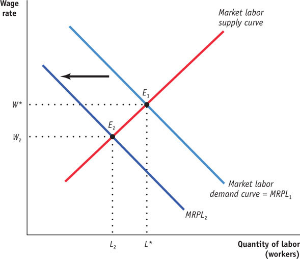
1. Draw a correctly labeled graph showing a perfectly competitive labor market in equilibrium. On your graph, label the labor demand curve, the labor supply curve, marginal revenue product of labor, the equilibrium wage (W*), and the equilibrium quantity of labor (L*).
2. Then, on the same graph, illustrate how a decrease in the price of the product made by the firm would affect the equilibrium wage and quantity of labor. Label the resulting wage rate W2 and the resulting quantity of labor L2.