1.3 3The Production Possibility Frontier Model
WHAT YOU WILL LEARN
 The importance of trade-offs in economic analysis
 What the production possibility frontier model tells us about efficiency, opportunity cost, and economic growth
 The two sources of economic growth—increases in the availability of resources and improvements in technology
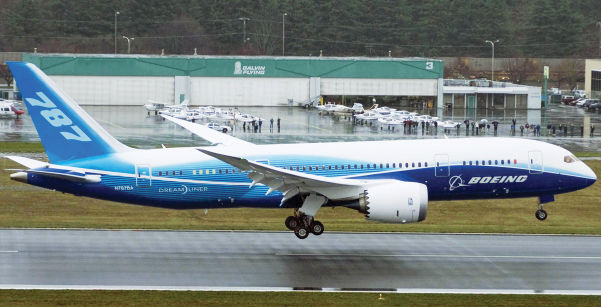
On December 15, 2009, Boeing’s newest jet, the 787 Dreamliner, took its first three-hour test flight. It was a historic moment: the Dreamliner was the result of an aerodynamic revolution—a superefficient airplane designed to cut airline operating costs and the first to use superlight composite materials. The jet underwent over 15,000 hours of wind tunnel tests that resulted in subtle design changes to improve its performance. Boeing engineers owe an enormous debt to the Wright brothers’ wind tunnel, which they used to model actual aircraft in flight. It made modern airplanes, including the Dreamliner, possible.
A good economic model can be a tremendous aid to understanding. In this module, we look at the production possibility frontier, a model that helps economists think about the trade-offs every economy faces. The production possibility frontier helps us understand three important aspects of the real economy: efficiency, opportunity cost, and economic growth.
Trade-offs: The Production Possibility Frontier
You make a trade-off when you give up something in order to have something else.
One of the important principles of economics we introduced in Module 1 was that resources are scarce. As a result, any economy—whether it contains one person or millions of people—faces trade-offs. You make a trade-off when you give up something in order to have something else. No matter how lightweight the Boeing Dreamliner is, and no matter how efficient Boeing’s assembly line, producing Dreamliners means using resources that therefore can’t be used to produce something else.
The production possibility frontier (PPF) illustrates the trade-offs facing an economy that produces only two goods. It shows the maximum quantity of one good that can be produced for each possible quantity of the other good produced.
To think about the trade-offs necessary in any economy, economists often use the production possibility frontier model. The idea behind this model is to improve our understanding of trade-offs by considering a simplified economy that produces only two goods. This simplification enables us to show the trade-offs graphically.
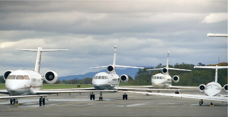
Suppose, for a moment, that the United States was a one-company economy, with Boeing its sole employer and aircraft its only product. But there would still be a choice of what kinds of aircraft to produce—say, Dreamliners versus small commuter jets.
Figure 3-1 shows a hypothetical production possibility curve representing the trade-off this one-company economy would face. The curve—the dark-blue line in the diagram—shows the maximum quantity of small jets that Boeing can produce per year given the quantity of Dreamliners it produces per year, and vice versa. That is, it answers questions of the form, “What is the maximum quantity of small jets that Boeing can produce in a year if it also produces Dreamliners that year?”
FIGURE3-1The Production Possibility Frontier
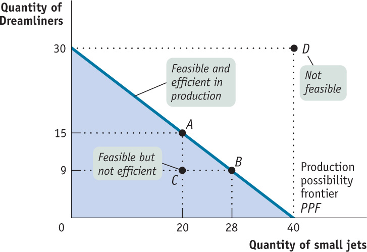
There is a crucial distinction between points inside or on the production possibility curve (the shaded area) and outside the curve. If a production point lies inside or on the curve—like point C, at which Boeing produces 20 small jets and 9 Dreamliners in a year—it is feasible. After all, the curve tells us that if Boeing produces 20 small jets, it could also produce a maximum of 15 Dreamliners that year, so it could certainly make 9 Dreamliners. However, a production point that lies outside the curve—such as the hypothetical production point D, where Boeing produces 40 small jets and 30 Dreamliners—isn’t feasible.
In Figure 3-1 the production possibility curve intersects the horizontal axis at 40 small jets. This means that if Boeing dedicated all its production capacity to making only small jets, it could produce 40 small jets per year. The production possibility curve intersects the vertical axis at 30 Dreamliners. This means that if Boeing dedicated all its production capacity to making Dreamliners, it could produce a maximum of 30 Dreamliners per year.
The figure also shows less extreme trade-offs. For example, if Boeing’s managers decide to make 20 small jets this year, they can produce at most 15 Dreamliners; this production choice is illustrated by point A. And if Boeing’s managers decide to produce 28 small jets, they can make at most 9 Dreamliners, as shown by point B.
Thinking in terms of a production possibility frontier simplifies the complexities of reality. The real-world U.S. economy produces millions of different goods. Even Boeing produces more than two different types of planes. Yet it’s important to realize that even in its simplicity, this stripped-down model gives us important insights about the real world.
By simplifying reality, the production possibility frontier helps us understand some aspects of the real economy better than we could without the model: efficiency, opportunity cost, and economic growth.
Efficiency
An economy is efficient if there is no way to make anyone better off without making anyone else worse off.
The production possibility frontier is useful for illustrating the general economic concept of efficiency. An economy is efficient if there are no missed opportunities—meaning that there is no way to make some people better off without making other people worse off. For example, suppose a course you are taking meets in a lecture hall or classroom that is too small for the number of students—some may be forced to sit on the floor or stand—despite the fact that a larger space nearby is empty during the same period. Economists would say that this is an inefficient use of resources because there is a way to make some people better off without making anyone worse off—after all, the larger space is empty. The school is not using its resources efficiently.
When an economy is using all of its resources efficiently, the only way one person can be made better off is by rearranging the use of resources in such a way that the change makes someone else worse off. So in our classroom example, if all larger classrooms or lecture halls were already fully occupied, we could say that the school was run in an efficient way; your classmates could be made better off only by making people in the larger classroom worse off—by moving them to the room that is too small.
Returning to our Boeing example, as long as Boeing operates on its production possibility curve, its production is efficient. At point A, 15 Dreamliners are the maximum quantity feasible given that Boeing has also committed to producing 20 small jets; at point B, 9 Dreamliners are the maximum number that can be made given the choice to produce 28 small jets; and so on.

But suppose for some reason that Boeing was operating at point C, making 20 small jets and 9 Dreamliners. In this case, it would not be operating efficiently and would therefore be inefficient: it could be producing more of both planes.
Another example of inefficiency in production occurs when people in an economy are involuntarily unemployed: they want to work but are unable to find jobs. When that happens, the economy is not efficient in production because it could produce more output if those people were employed. The production possibility frontier shows the amount that can possibly be produced if all resources are fully employed. In other words, changes in unemployment move the economy closer to, or further away from, the PPF. But the curve itself is determined by what would be possible if there were full employment in the economy. Greater unemployment is represented by points farther below the PPF—the economy is not reaching its possibilities if it is not using all of its resources. Lower unemployment is represented by points closer to the PPF—as unemployment decreases, the economy moves closer to reaching its possibilities.
Although the production possibility frontier helps clarify what it means for an economy to be efficient in production, it’s important to understand that efficiency in production is only part of what’s required for the economy as a whole to be efficient. Efficiency also requires that the economy allocate its resources so that consumers are as well off as possible. If an economy does this, we say that it is efficient in allocation.
To see why efficiency in allocation is as important as efficiency in production, notice that points A and B in Figure 3-1 both represent situations in which the economy is efficient in production, because in each case it can’t produce more of one good without producing less of the other. But these two situations may not be equally desirable. It may be more desirable to have more small jets and fewer Dreamliners than at point A; such as 28 small jets and 9 Dreamliners, corresponding to point B. In this case, point A is inefficient from the point of view of the economy as a whole: it is possible to move from point A to point B, and have some be made better off without making anyone else worse off.
This example shows that efficiency for the economy as a whole requires both efficiency in production and efficiency in allocation. To be efficient, an economy must produce as much of each good as it can, given the production of other goods, and it must also produce the mix of goods that people want to consume.
Opportunity Cost
The production possibility frontier is also useful as a reminder that the true cost of any good isn’t the money it costs to buy, but what must be given up in order to get that good—the opportunity cost. If, for example, Boeing decides to change its production from point A to point B, it will produce 8 more small jets but 6 fewer Dreamliners. So the opportunity cost of 8 small jets is 6 Dreamliners—the 6 Dreamliners that can’t be produced if Boeing produces 8 more small jets. This means that each small jet has an opportunity cost of  = ¾ of a Dreamliner.
Is the opportunity cost of an extra small jet in terms of Dreamliners always the same, no matter how many small jets and Dreamliners are currently produced? In the example illustrated by Figure 3-1, the answer is yes. If Boeing increases its production of small jets from 28 to 40, the number of Dreamliners it produces falls from 9 to zero. So Boeing’s opportunity cost per additional small jet is  = ¾ of a Dreamliner, the same as it was when Boeing went from 20 small jets produced to 28. The fact that the opportunity cost is always the same number—¾ in this case—is just one possible assumption we could make in this case. Anytime we make the assumption that the opportunity cost of an additional unit of a good doesn’t change regardless of the output mix, the production possibilities curve is drawn as a straight line, as it is in Figure 3-1.
Moreover, as you might have already guessed, the slope of a straight-line production possibility curve is equal to the opportunity cost—specifically, the opportunity cost for the good measured on the horizontal axis in terms of the good measured on the vertical axis. In Figure 3-1, the production possibility curve has a constant slope of −¾, implying that Boeing faces a constant opportunity cost for 1 small jet equal to ¾ of a Dreamliner. (A review of how to calculate the slope of a straight line is found in Appendix A at the back of the book.) This is the simplest case, but the production possibility frontier model can also be used to examine situations in which opportunity costs change as the mix of output changes.
Figure 3-2 illustrates a different assumption, a case in which Boeing faces increasing opportunity cost. Here, the more small jets it produces, the more costly it is to produce yet another small jet in terms of reduced production of a Dreamliner. For example, to go from producing zero small jets to producing 20, Boeing has to give up producing 5 Dreamliners. That is, the opportunity cost of those 20 small jets is 5 Dreamliners. But to increase its production of small jets to 40—that is, to produce an additional 20 small jets—it must produce 25 fewer Dreamliners, a much higher opportunity cost. And the same holds true in reverse: the more Dreamliners Boeing produces, the more costly it is to produce yet another Dreamliner in terms of reduced production of small jets. As you can see in Figure 3-2, when opportunity costs are increasing rather than constant, the production possibility curve is bowed outward rather than a straight line.
FIGURE3-2Increasing Opportunity Cost
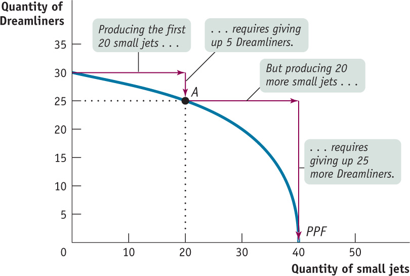
Although it’s often useful to work with the simple assumption that the production possibility curve is a straight line, economists believe that in reality, opportunity costs are typically increasing. When only a small amount of a good is produced, the opportunity cost of producing that good is relatively low because the economy needs to use only those resources that are especially well suited for its production. For example, if an economy grows only a small amount of corn, that corn can be grown in places where the soil and climate are perfect for growing corn but less suitable for growing anything else, such as wheat.
So growing that corn involves giving up only a small amount of potential wheat output. Once the economy grows a lot of corn, however, land that is well suited for wheat but isn’t so great for corn must be used to produce corn anyway. As a result, the additional corn production involves sacrificing considerably more wheat production. In other words, as more of a good is produced, its opportunity cost typically rises because well-suited inputs are used up and less adaptable inputs must be used instead.
Economic Growth
Finally, the production possibility frontier helps us understand what it means to talk about economic growth, which economists describe as creating a sustained rise in aggregate output. Economic growth is one of the fundamental features of the economy. But are we really justified in saying that the economy has grown over time? After all, although the U.S. economy produces more of many things than it did a century ago, it produces less of other things—for example, horse-drawn carriages. In other words, production of many goods is actually down. So how can we say for sure that the economy as a whole has grown?
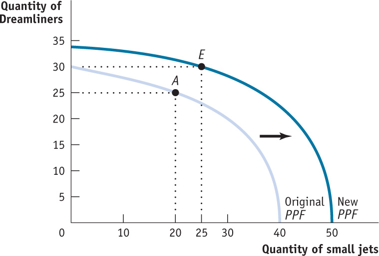
The answer, illustrated in Figure 3-3, is that economic growth means an expansion of the economy’s production possibilities: the economy can produce more of everything. In it, we assume again that our economy is only made up of Boeing, and therefore, our economy only produces two goods, Dreamliners and small jets. For example, if Boeing’s production is initially at point A (20 small jets and 25 Dreamliners) economic growth means that Boeing could move to point E (25 small jets and 30 Dreamliners). Point E lies outside the original curve, so in the production possibility frontier model, growth is shown as an outward shift of the curve.
FIGURE3-3Economic Growth
Factors of production are resources used to produce goods and services.
What can lead the production possibility curve to shift outward? There are basically two sources of economic growth. One is an increase in the economy’s factors of production, the resources used to produce goods and services. Broadly speaking, the main factors of production are the resources land, labor, physical capital, and human capital. As you learned in Module 1, land is a resource supplied by nature; labor is the economy’s pool of workers; physical capital refers to created resources such as machines and buildings; and human capital refers to the educational achievements and skills of the labor force, which enhance its productivity.
To see how adding to an economy’s factors of production leads to economic growth, suppose that Boeing builds another construction hangar that allows it to increase the number of planes—small jets or Dreamliners or both—it can produce in a year. The new construction hangar is a factor of production, a resource Boeing can use to increase its yearly output. We can’t say how many more planes of each type Boeing will produce; that’s a management decision that will depend on, among other things, customer demand. But we can say that Boeing’s production possibility curve has shifted outward because it can now produce more small jets without reducing the number of Dreamliners it makes, or it can make more Dreamliners without reducing the number of small jets produced.

Comstock/Thinkstock
iStockphoto/Thinkstock
iStockphoto/Thinkstock
Technology is the technical means for producing goods and services.
The other source of economic growth is progress in technology, the technical means for the production of goods and services. Composite materials had been used in some parts of aircraft before the Boeing Dreamliner was developed. But Boeing engineers realized that there were large additional advantages to building a whole plane out of composites. The plane would be lighter, stronger, and have better aerodynamics than a plane built in the traditional way. It would therefore have longer range, be able to carry more people, and use less fuel, in addition to being able to maintain higher cabin pressure. So in a real sense Boeing’s innovation—a whole plane built out of composites—was a way to do more with any given amount of resources, pushing out the production possibility curve.
But even if, for some reason, Boeing chooses to produce either fewer Dreamliners or fewer small jets than before, we would still say that this economy has grown, because it could have produced more of everything. At the same time, if an economy’s production possibility curve shifts inward, the economy has become smaller. This could happen if the economy loses resources or technology (for example, if it experiences war or a natural disaster).
The production possibility frontier is a very simplified model of an economy. Yet it teaches us important lessons about real-world economies. It gives us our first clear sense of what constitutes economic efficiency, it illustrates the concept of opportunity cost, and it makes clear what economic growth is all about.
3
Solutions appear at the back of the book.
Check Your Understanding
1. True or false? Explain your answer.
-
a. An increase in the amount of resources available to Boeing for use in producing Dreamliners and small jets does not change its production possibility curve.
False. An increase in the resources available to Boeing for use in producing Dreamliners and small jets changes the production possibility curve by shifting it outward. This is because Boeing can now produce more small jets and Dreamliners than before. In the accompanying figure, the line labeled “Boeing’s original PPF” represents Boeing’s original production possibility curve, and the line labeled “Boeing’s new PPF” represents the new production possibility curve that results from an increase in resources available to Boeing.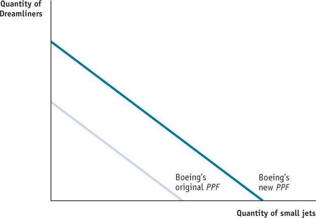
-
b. A technological change that allows Boeing to build more small jets for any amount of Dreamliners built results in a change in its production possibility curve.
True. A technological change that allows Boeing to build more small jets for any amount of Dreamliners built results in a change in its production possibility curve. This is illustrated in the accompanying figure: the new production possibility curve is represented by the line labeled “Boeing’s new PPF,” and the original production curve is represented by the line labeled “Boeing’s original PPF.” Since the maximum quantity of Dreamliners that Boeing can build is the same as before, the new production possibility curve intersects the vertical axis at the same point as the original curve. But since the maximum possible quantity of small jets is now greater than before, the new curve intersects the horizontal axis to the right of the original curve.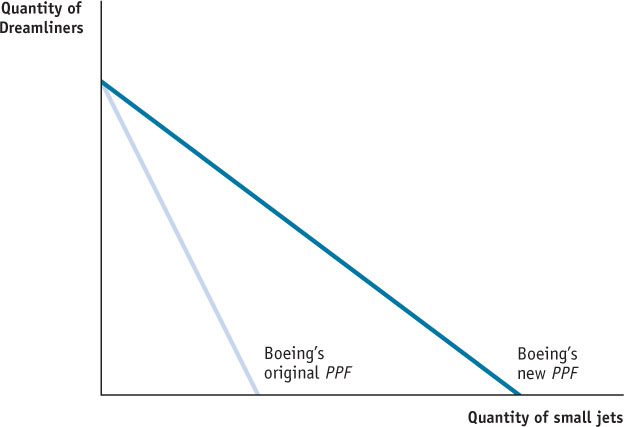
-
c. The production possibility frontier is useful because it illustrates how much of one good an economy must give up to get more of another good regardless of whether resources are being used efficiently.
False. The production possibility frontier illustrates how much of one good an economy must give up to get more of another good only when resources are used efficiently in production. If an economy is producing inefficiently— that is, inside the frontier—then it does not have to give up a unit of one good in order to get another unit of the other good. Instead, by becoming more efficient in production, this economy can have more of both goods.
Multiple-Choice Questions
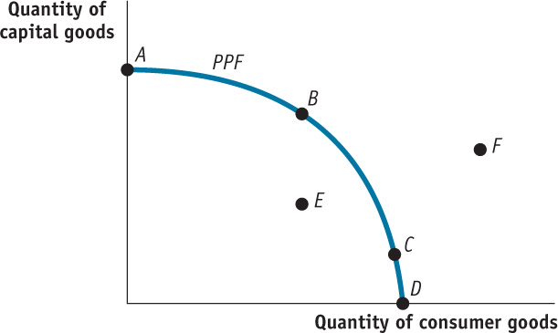
Refer to the accompanying graph to answer the following questions.
Question
1. Which point(s) on the graph represent efficiency in production?
| A. |
| B. |
| C. |
| D. |
| E. |
Question
2. For this economy, an increase in the quantity of capital goods produced without a corresponding decrease in the quantity of consumer goods produced
| A. |
| B. |
| C. |
| D. |
| E. |
Question
3. An increase in unemployment could be represented by a movement from point
| A. |
| B. |
| C. |
| D. |
| E. |
Question
4. Which of the following might allow this economy to move from point B to point F?
| A. |
| B. |
| C. |
| D. |
| E. |
Question
5. This production possibility curve shows the trade-off between consumer goods and capital goods. Since capital goods are a resource, an increase in the production of capital goods today will increase the economy’s production possibilities in the future. Therefore, all other things being equal, producing at which point today will result in the largest outward shift of the PPF in the future?
| A. |
| B. |
| C. |
| D. |
| E. |
Critical-Thinking Questions
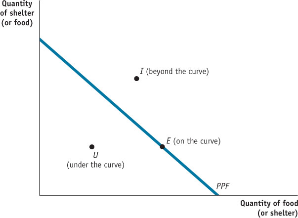
Assume that an economy can choose between producing food and producing shelter at a constant opportunity cost. Graph a correctly labeled production possibility curve for the economy. On your graph:
1. Use the letter E to label one of the points that is efficient in production.
2. Use the letter U to label one of the points at which there might be unemployment.
3. Use the letter I to label one of the points that is not feasible.
