1.1 8Income Effects, Substitution Effects, and Elasticity

© Monkey Business Images/Dreamstime.com

Explaining the Law of Demand

We introduced the demand curve and the law of demand in the previous section on supply and demand. To this point, we have accepted that the demand curve has a negative slope. And we have drawn demand curves that are somewhere in the middle between flat and steep (with a negative slope). In this module, we present more detail about why demand curves slope downward and what the slope of the demand curve tells us. We begin with the income and substitution effects, which explain why the demand curve has a negative slope.

The Substitution Effect

When the price of a good increases, an individual will normally consume less of that good and more of other goods. Correspondingly, when the price of a good decreases, an individual will normally consume more of that good and less of other goods. This explains why the individual demand curve, which relates an individual’s consumption of a good to the price of that good, normally slopes downward—that is, it obeys the law of demand.

An alternative way to think about why demand curves slope downward is to focus on opportunity costs. For simplicity, let’s suppose there are only two goods between which to choose. When the price of one good decreases, an individual doesn’t have to give up as many units of the other good in order to buy one more unit of the first good. That makes it attractive to buy more of the good whose price has gone down. Conversely, when the price of one good increases, one must give up more units of the other good to buy one more unit of the first good, so consuming that good becomes less attractive and the consumer buys fewer.

The change in the quantity demanded as the good that has become relatively cheaper is substituted for the good that has become relatively more expensive is known as the substitution effect. When a good absorbs only a small share of the typical consumer’s income, as with pillow cases and swim goggles, the substitution effect is essentially the sole explanation of why the market demand curve slopes downward. There are, however, some goods, like food and housing, that account for a substantial share of many consumers’ incomes. In such cases another effect, called the income effect, also comes into play.

The Income Effect

Consider the case of a family that spends half of its income on rental housing. Now suppose that the price of housing increases everywhere. This will have a substitution effect on the family’s demand: other things equal, the family will have an incentive to consume less housing—say, by moving to a smaller apartment—and more of other goods. But the family will also, in a real sense, be made poorer by that higher housing price—its income will buy less housing than before.

When income is adjusted to reflect its true purchasing power, it is called real income, in contrast to money income or nominal income, which has not been adjusted. And this reduction in a consumer’s real income will have an additional effect, beyond the substitution effect, on the family’s consumption choices, including its consumption of housing. The income effect is the change in the quantity of a good demanded that results from a change in the overall purchasing power of the consumer’s income due to a change in the price of that good.

It’s possible to give more precise definitions of the substitution effect and the income effect of a price change, but for most purposes, there are only two things you need to know about the distinction between these two effects.

1. For the majority of goods and services, the income effect is not important and has no significant effect on individual consumption. Thus, most market demand curves slope downward solely because of the substitution effect—end of story.
2. When it matters at all, the income effect usually reinforces the substitution effect. That is, when the price of a good that absorbs a substantial share of income rises, consumers of that good become a bit poorer because their purchasing power falls. And the vast majority of goods are normal goods, goods for which demand decreases when income falls. So this effective reduction in income leads to a reduction in the quantity demanded and reinforces the substitution effect.

However, in the case of an inferior good, a good for which demand increases when income falls, the income and substitution effects work in opposite directions. Although the substitution effect decreases the quantity of any good demanded as its price increases, the income effect of a price increase for an inferior good is an increase in the quantity demanded. This makes sense because the price increase lowers the real income of the consumer, and as real income falls, the demand for an inferior good increases.

If a good were so inferior that the income effect exceeded the substitution effect, a price increase would lead to an increase in the quantity demanded. There is controversy over whether such goods, known as “Giffen goods,” exist at all. (See the following Economics in Action for more on “Giffen goods”). If they do, they are very rare. You can generally assume that the income effect for an inferior good is smaller than the substitution effect, and so a price increase will still lead to a decrease in the quantity demanded.

GIFFEN GOODS

Two hundred years ago, when Ireland was under British rule and desperately poor, it was claimed that the Irish would eat more potatoes when the price of potatoes went up. That is, some observers claimed that Ireland’s demand curve for potatoes sloped upward, not downward.

Can this happen? In theory, yes. If Irish demand for potatoes actually sloped upward, it would have been a real-life case of a “Giffen good,” named after a nineteenth-century statistician who thought (probably wrongly) that he saw an upward-sloping demand curve in some data he was studying.

Here’s the story. Suppose that there is some good that absorbs a large share of consumers’ budgets and that this good is also inferior—people demand less of it when their income rises. The classic supposed example was, as you might guess, potatoes in Ireland, back when potatoes were an inferior good—they were what poor people ate—and when the Irish were very poor.

iStockphoto/Thinkstock

Now suppose that the price of potatoes increases. This would, other things being equal, cause people to substitute other goods for potatoes. But other things are not equal: given the higher price of potatoes, people are poorer. And this increases the demand for potatoes, because potatoes are an inferior good.

If this income effect outweighs the substitution effect, a rise in the price of potatoes would increase the quantity demanded; the law of demand would not hold.

In a way the point of this story—which has never been validated in any real situation, nineteenth-century Ireland included—is how unlikely such an event is. The law of demand really is a law, with few exceptions.

Defining and Measuring Elasticity

Most graphs in economics depict relationships between two variables: the value of one determining variable (the independent variable) directly influences the value of the other (the dependent variable). If two variables are negatively related and the independent variable increases, the dependent variable will respond by decreasing. (For a review of graphing variables, see Appendix A on graphs in economics, at the back of the book.) But often the important question is not whether the variables are negatively or positively related, but how responsive the dependent variable is to changes in the independent variable (that is, by how much will the dependent variable change?). If price increases, we know that quantity demanded will decrease (that is the law of demand). The question in this context is by how much will quantity demanded decrease if price goes up?

Economists use the concept of elasticity to measure the responsiveness of one variable to changes in another. For example, price elasticity of demand measures the responsiveness of quantity demanded to changes in price—something a firm considering changing its price would certainly want to know! Elasticity can be used to measure responsiveness using any two related variables. We will start by looking at the price elasticity of demand and then move on to other examples of elasticities commonly used by economists.

Think back to the opening story of the 2004 flu shot panic. In order for Flunomics, a hypothetical flu vaccine distributor, to know whether it could raise its revenue by significantly raising the price of its flu vaccine during the 2004 flu vaccine panic, it would have to know whether the price increase would decrease the quantity demanded by a lot or a little. That is, it would have to know the price elasticity of demand for flu vaccinations.

Calculating the Price Elasticity of Demand

Figure 8-1 shows a hypothetical demand curve for flu vaccinations. At a price of $20 per vaccination, consumers would demand 10 million vaccinations per year (point A); at a price of $21, the quantity demanded would fall to 9.9 million vaccinations per year (point B).

FIGURE8-1The Demand for Vaccinations

At a price of $20 per vaccination, the quantity of vaccinations demanded is 10 million per year (point A). When price rises to $21 per vaccination, the quantity demanded falls to 9.9 million vaccinations per year (point B).

Figure 8-1, then, tells us the change in the quantity demanded for a particular change in the price. But how can we turn this into a measure of price responsiveness? The answer is to calculate the price elasticity of demand. The price elasticity of demand compares the percent change in quantity demanded to the percent change in price as we move along the demand curve. As we’ll see later, the reason economists use percent changes is to get a measure that doesn’t depend on the units in which a good is measured (say, a child-size dose versus an adult-size dose of vaccine). But before we get to that, let’s look at how elasticity is calculated.

To calculate the price elasticity of demand, we first calculate the percent change in the quantity demanded and the corresponding percent change in the price as we move along the demand curve. These are defined as follows:

and

In Figure 8-1, we see that when the price rises from $20 to $21, the quantity demanded falls from 10 million to 9.9 million vaccinations, yielding a change in the quantity demanded of 0.1 million vaccinations. So the percent change in the quantity demanded is

The initial price is $20 and the change in the price is $1, so the percent change in the price is

To calculate the price elasticity of demand, we find the ratio of the percent change in the quantity demanded to the percent change in the price:

In Figure 8-1, the price elasticity of demand is therefore

Notice that the minus sign has been dropped from this equation. Why have we done this?

The law of demand says that demand curves slope downward, so price and quantity demanded always move in opposite directions. In other words, a positive percent change in price (a rise in price) leads to a negative percent change in the quantity demanded; a negative percent change in price (a fall in price) leads to a positive percent change in the quantity demanded. This means that the price elasticity of demand is, in strictly mathematical terms, a negative number. However, it is inconvenient to repeatedly write a minus sign. So when economists talk about the price elasticity of demand, they usually drop the minus sign and report the absolute value of the price elasticity of demand. In other words, the absolute value of a negative number appears without the minus sign. In this case, for example, economists would usually say “the price elasticity of demand is 0.2,” taking it for granted that you understand they mean minus 0.2. We follow this convention here.

The larger the price elasticity of demand, the more responsive the quantity demanded is to the price. When the price elasticity of demand is large—when consumers change their quantity demanded by a large percentage compared to the percent change in the price—economists say that demand is highly elastic.

As we’ll see shortly, a price elasticity of 0.2 indicates a small response of quantity demanded to price. That is, the quantity demanded will fall by a relatively small amount when price rises. This is what economists call inelastic demand. And inelastic demand was exactly what Flunomics needed for its strategy to increase revenue by raising the price of its flu vaccines.

An Alternative Way to Calculate Elasticities: The Midpoint Method

We’ve seen that price elasticity of demand compares the percent change in quantity demanded with the percent change in price. When we look at some other elasticities, which we will do shortly, we’ll see why it is important to focus on percent changes. But at this point we need to discuss a technical issue that arises when you calculate percent changes in variables and how economists deal with it.

The best way to understand the issue is with a real example. Suppose you were trying to estimate the price elasticity of demand for gasoline by comparing gasoline prices and consumption in different countries. Because of high taxes, gasoline usually costs about three times as much per gallon in Europe as it does in the United States. So what is the percent difference between American and European gas prices?

Well, it depends on which way you measure it. Because the price of gasoline in Europe is approximately three times higher than in the United States, it is 200 percent higher. Because the price of gasoline in the United States is one-third as high as in Europe, it is 66.7 percent lower.

© Dan Van Den Broeke/Dreamstime.com

This is a nuisance: we’d like to have a percent measure of the difference in prices that doesn’t depend on which way you measure it. A good way to avoid computing different elasticities for rising and falling prices is to use the midpoint method (sometimes called the arc method).

The midpoint method replaces the usual definition of the percent change in a variable, X, with a slightly different definition:

where the average value of X is defined as

When calculating the price elasticity of demand using the midpoint method, both the percent change in the price and the percent change in the quantity demanded are found using average values in this way. To see how this method works, suppose you have the following data for some good:

To calculate the percent change in quantity going from situation A to situation B, we compare the change in the quantity demanded—a fall of 200 units—with the average of the quantity demanded in the two situations. So we calculate

In the same way, we calculate the percent change in price as

So in this case we would calculate the price elasticity of demand to be

again dropping the minus sign.

The important point is that we would get the same result, a price elasticity of demand of 1, whether we went up the demand curve from situation A to situation B or down from situation B to situation A.

To arrive at a more general formula for price elasticity of demand, suppose that we have data for two points on a demand curve. At point 1 the quantity demanded and price are (Q₁, P₁); at point 2 they are (Q₂, P₂). Then the formula for calculating the price elasticity of demand is:

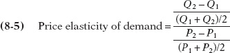
As before, when reporting a price elasticity of demand calculated by the midpoint method, we drop the minus sign and report the absolute value.

8

Check Your Understanding

1. In each of the following cases, state whether the income effect, the substitution effect, or both are significant. In which cases do they move in the same direction? In opposite directions? Why?

• a. Orange juice represents a small share of Clare’s spending. She buys more lemonade and less orange juice when the price of orange juice goes up. She does not change her spending on other goods.

  Since spending on orange juice is a small share of Clare’s spending, the income effect from a rise in the price of orange juice is insignificant. Only the substitution effect, represented by the substitution of lemonade for orange juice, is significant.

• b. Apartment rents have risen dramatically this year. Since rent absorbs a major part of her income, Delia moves to a smaller apartment. Assume that rental housing is a normal good.

  Since rent is a large share of Delia’s expenditures, the increase in rent generates an income effect, making Delia feel poorer. Since housing is a normal good for Delia, the income and substitution effects move in the same direction, leading her to reduce her consumption of housing by moving to a smaller apartment.

• c. The cost of a semester-long meal ticket at the student cafeteria rises, representing a significant increase in living costs. As a result, many students have less money to spend on weekend meals at restaurants and eat in the cafeteria instead. Assume that cafeteria meals are an inferior good.

  Since a meal ticket is a significant share of the students’ living costs, an increase in its price will generate an income effect. Students respond to the price increase by eating more often in the cafeteria. So the substitution effect (which would induce them to eat in the cafeteria less often as they substitute restaurant meals in place of meals at the cafeteria) and the income effect (which would induce them to eat in the cafeteria more often because they are poorer) move in opposite directions. This happens because cafeteria meals are an inferior good. In fact, since the income effect outweighs the substitution effect (students eat in the cafeteria more as the price of meal tickets increases), cafeteria meals are a Giffen good.

2. The price of strawberries falls from $1.50 to $1.00 per carton, and the quantity demanded goes from 100,000 to 200,000 cartons. Use the midpoint method to find the price elasticity of demand.

By the midpoint method, the percent change in the quantity of strawberries demanded is

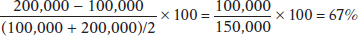
Similarly, the percent change in the price of strawberries is

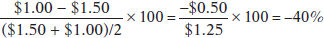
Dropping the minus sign, the price elasticity of demand using the midpoint method is 67%/40% = 1.7.

3. At the present level of consumption, 4,000 movie tickets, and at the current price, $5 per ticket, the price elasticity of demand for movie tickets is 1. Using the midpoint method, calculate the percentage by which the owners of movie theaters must reduce the price in order to sell 5,000 tickets.

By the midpoint method, the percent change in the quantity of movie tickets demanded in going from 4,000 tickets to 5,000 tickets is

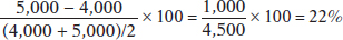
Since the price elasticity of demand is 1 at the current consumption level, it will take a 22% reduction in the price of movie tickets to generate a 22% increase in quantity demanded.

4. The price elasticity of demand for ice-cream sandwiches is 1.2 at the current price of $0.50 per sandwich and the current consumption level of 100,000 sandwiches. Calculate the change in the quantity demanded when price rises by $0.05. Use Equations 8-1 and 8-2 to calculate percent changes and Equation 8-3 to relate price elasticity of demand to the percent changes.

Since price rises, we know that quantity demanded must fall. Given the current price of $0.50, a $0.05 increase in price represents a 10% change, using the method in Equation 8-2. So the price elasticity of demand is

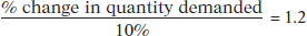
so that the percent change in quantity demanded is 12%. A 12% decrease in quantity demanded represents 100,000 × 0.12, or 12,000 sandwiches.

Assume the price of an inferior good increases.