1.3 10Other Elasticities

(left) Msheldrake/Dreamstime.com
(right) © Lauri Pattersoni/iStockphoto

Using Other Elasticities

We stated earlier that economists use the concept of elasticity to measure the responsiveness of one variable to changes in another. However, up to this point we have focused on the price elasticity of demand. Now that we have used elasticity to measure the responsiveness of quantity demanded to changes in price, we can go on to look at how elasticity is used to understand the relationship between other important variables in economics.

The quantity of a good demanded depends not only on the price of that good but also on other variables. In particular, demand curves shift because of changes in the prices of related goods and changes in consumers’ incomes. It is often important to have a measure of these other effects, and the best measures are—you guessed it—elasticities. Specifically, we can best measure how the demand for a good is affected by prices of other goods using a measure called the cross-price elasticity of demand, and we can best measure how demand is affected by changes in income using the income elasticity of demand.

Finally, we can also use elasticity to measure supply responses. The price elasticity of supply measures the responsiveness of the quantity supplied to changes in price.

The Cross-Price Elasticity of Demand

The demand for a good is often affected by the prices of other, related goods—goods that are substitutes or complements. A change in the price of a related good shifts the demand curve of the original good, reflecting a change in the quantity demanded at any given price. The strength of such a “cross” effect on demand can be measured by the cross-price elasticity of demand, defined as the ratio of the percent change in the quantity demanded of one good to the percent change in the price of another.

When two goods are substitutes, like hot dogs and hamburgers, the cross-price elasticity of demand is positive: a rise in the price of hot dogs increases the demand for hamburgers—that is, it causes a rightward shift of the demand curve for hamburgers. If the goods are close substitutes, the cross-price elasticity will be positive and large; if they are not close substitutes, the cross-price elasticity will be positive and small. So when the cross-price elasticity of demand is positive, its size is a measure of how closely substitutable the two goods are, with a higher number meaning the goods are closer substitutes.

When two goods are complements, like hot dogs and hot dog buns, the cross-price elasticity is negative: a rise in the price of hot dogs decreases the demand for hot dog buns—that is, it causes a leftward shift of the demand curve for hot dog buns. As with substitutes, the size of the cross-price elasticity of demand between two complements tells us how strongly complementary they are: if the cross-price elasticity is only slightly below zero, they are weak complements; if it is very negative, they are strong complements.

Note that in the case of the cross-price elasticity of demand, the sign (plus or minus) is very important: it tells us whether the two goods are complements or substitutes. So we cannot drop the minus sign as we did for the price elasticity of demand.

Our discussion of the cross-price elasticity of demand is a useful place to return to a point we made earlier: elasticity is a unit-free measure—that is, it doesn’t depend on the units in which goods are measured.

To see the potential problem, suppose someone told you that “if the price of hot dog buns rises by $0.30, Americans will buy 10 million fewer hot dogs this year.” If you’ve ever bought hot dog buns, you’ll immediately wonder: is that a $0.30 increase in the price per bun, or is it a $0.30 increase in the price per package of buns? It makes a big difference what units we are talking about! However, if someone says that the cross-price elasticity of demand between buns and hot dogs is −0.3, it doesn’t matter whether buns are sold individually or by the package. So elasticity is defined as a ratio of percent changes, which avoids confusion over units.

The Income Elasticity of Demand

The income elasticity of demand measures how changes in income affect the demand for a good. It indicates whether a good is normal or inferior and specifies how responsive demand for the good is to changes in income. Having learned the price and cross-price elasticity formulas, the income elasticity formula will look familiar:

Just as the cross-price elasticity of demand between two goods can be either positive or negative, depending on whether the goods are substitutes or complements, the income elasticity of demand for a good can also be either positive or negative. Recall that goods can be either normal goods, for which demand increases when income rises, or inferior goods, for which demand decreases when income rises. These definitions relate directly to the sign of the income elasticity of demand:

• When the income elasticity of demand is positive, the good is a normal good—that is, the quantity demanded at any given price increases as income increases.
• When the income elasticity of demand is negative, the good is an inferior good—that is, the quantity demanded at any given price decreases as income increases.

Economists often use estimates of the income elasticity of demand to predict which industries will grow most rapidly as the incomes of consumers grow over time. In doing this, they often find it useful to make a further distinction among normal goods, identifying which are income-elastic and which are income-inelastic.

The demand for a good is income-elastic if the income elasticity of demand for that good is greater than 1. When income rises, the demand for income-elastic goods rises faster than income. Luxury goods such as second homes and international travel tend to be income-elastic. The demand for a good is income-inelastic if the income elasticity of demand for that good is positive but less than 1. When income rises, the demand for income-inelastic goods rises, but more slowly than income. Necessities such as food and clothing tend to be income-inelastic.

WILL CHINA SAVE THE U.S. FARMING SECTOR?

In the days of the Founding Fathers, the great majority of Americans lived on farms. As recently as the 1940s, one American in six—or approximately 17%—still did. But in 2007, the official number was less than 1%. Why do so few people now live and work on farms in the United States? There are two main reasons, both involving elasticities.

First, the income elasticity of demand for food is much less than 1—it is income-inelastic. As consumers grow richer, other things being equal, spending on food rises less than income. As a result, as the U.S. economy has grown, the share of income it spends on food—and therefore the share of total U.S. income earned by farmers—has fallen.

Second, the demand for food is price-inelastic. This is important because technological advances in American agriculture have steadily raised yields over time and led to a long-term trend of lower U.S. food prices for most of the past century and a half. The combination of price inelasticity and falling prices led to falling total revenue for farmers. That’s right: progress in farming has been good for American consumers but bad for American farmers.

Why do so few Americans live and work on farms?

Cultura Limited/SuperStock

The combination of these effects explains the long-term relative decline of farming in the United States. The low income elasticity of demand for food ensures that the income of farmers grows more slowly than the economy as a whole. And the combination of rapid technological progress in farming with price-inelastic demand for foodstuffs reinforces this effect, further reducing the growth of farm income.

That is, up until now. Starting in the mid-2000s, increased demand for foodstuffs from rapidly growing developing countries like China has pushed up the prices of agricultural products around the world. And American farmers have benefited, with U.S. farm net income rising 47% in 2011 alone. Eventually, as the growth in developing countries tapers off and agricultural innovation continues to progress, it’s likely that the agricultural sector will resume its downward trend. But for now and for the foreseeable future, American farmers are enjoying the sector’s revival.

The Price Elasticity of Supply

In the wake of the flu vaccine shortfall of 2004, attempts by vaccine distributors to drive up the price of vaccines would have been much less effective if a higher price had induced a large increase in the output of flu vaccines by flu vaccine manufacturers other than Chiron. In fact, if the rise in price had precipitated a significant increase in flu vaccine production, the price would have been pushed back down. But that didn’t happen because, as we mentioned earlier, it would have been far too costly and technically difficult to produce more vaccine for the 2004–2005 flu season. (In reality, the production of flu vaccine is begun a year before it is to be distributed.)

This was another critical element in the ability of some flu vaccine distributors, like Med-Stat, to get significantly higher prices for their product: a low responsiveness in the quantity of output supplied to the higher price of flu vaccine by flu vaccine producers. To measure the response of producers to price changes, we need a measure parallel to the price elasticity of demand—the price elasticity of supply.

Measuring the Price Elasticity of Supply

The price elasticity of supply is defined the same way as the price elasticity of demand (although there is no minus sign to be eliminated here):

The only difference is that now we consider movements along the supply curve rather than movements along the demand curve.

Suppose that the price of tomatoes rises by 10%. If the quantity of tomatoes supplied also increases by 10% in response, the price elasticity of supply of tomatoes is 1 (10%/10%) and supply is unit-elastic. If the quantity supplied increases by 5%, the price elasticity of supply is 0.5 and supply is inelastic; if the quantity supplied increases by 20%, the price elasticity of supply is 2 and supply is elastic.

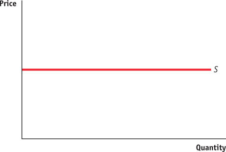
FIGURE10-1Two Extreme Cases of Price Elasticity of Supply

Panel (a) shows a perfectly inelastic supply curve, which is a vertical line. The price elasticity of supply is zero: the quantity supplied is always the same, regardless of price. Panel (b) shows a perfectly elastic supply curve, which is a horizontal line. At a price of $12, producers will supply any quantity, but they will supply none at a price below $12. If the price rises above $12, they will supply an extremely large quantity.

As with the demand side, the extreme values of the price elasticity of supply have a simple graphical representation. Panel (a) of Figure 10-1 shows the supply of cell phone frequencies, the portion of the radio spectrum that is suitable for sending and receiving cell phone signals. Governments own the right to sell the use of this part of the radio spectrum to cell phone operators inside their borders. But governments can’t increase or decrease the number of cell phone frequencies they have to offer—for technical reasons, the quantity of frequencies suitable for cell phone operation is fixed.

So the supply curve for cell phone frequencies is a vertical line, which we have assumed is set at the quantity of 100 frequencies. As you move up and down that curve, the change in the quantity supplied by the government is zero, whatever the change in price. So panel (a) illustrates a case of perfectly inelastic supply, meaning that the price elasticity of supply is zero.

The price elasticity of supply for pizza is very high because the inputs needed to make more of it are readily available.

Dehooks/Dreamstime.com

Panel (b) shows the supply curve for pizza. We suppose that it costs $12 to produce a pizza, including all opportunity costs. At any price below $12, it would be unprofitable to produce pizza and all the pizza parlors would go out of business. At a price of $12 or more, there are many producers who could operate pizza parlors. The ingredients—flour, tomatoes, cheese—are plentiful. And if necessary, more tomatoes could be grown, more milk could be produced to make mozzarella cheese, and so on. So by allowing profits, any price above $12 would elicit the supply of an extremely large quantity of pizzas. The implied supply curve is therefore a horizontal line at $12.

Since even a tiny increase in the price would lead to an enormous increase in the quantity supplied, the price elasticity of supply would be virtually infinite. A horizontal supply curve such as this represents a case of perfectly elastic supply.

As our cell phone frequencies and pizza examples suggest, real-world instances of both perfectly inelastic and perfectly elastic supply are easier to find than their counterparts in demand.

What Factors Determine the Price Elasticity of Supply?

Our examples tell us the main determinant of the price elasticity of supply: the availability of inputs. In addition, as with the price elasticity of demand, time may also play a role in the price elasticity of supply. Here we briefly summarize the two factors.

The Availability of InputsThe price elasticity of supply tends to be large when inputs are readily available and can be shifted into and out of production at a relatively low cost. It tends to be small when inputs are available only in a more-or-less fixed quantity or can be shifted into and out of production only at a relatively high cost.

TimeThe price elasticity of supply tends to grow larger as producers have more time to respond to a price change. This means that the long-run price elasticity of supply is often higher than the short-run elasticity. In the case of the flu vaccine shortfall, time was the crucial element because flu vaccine must be grown in cultures over many months.

The price elasticity of supply is usually less than perfectly elastic for goods, such as ocean fish, that are limited natural resources.

istockphoto

The price elasticity of the supply of pizza is very high because the inputs needed to make more pizza are readily available. The price elasticity of cell phone frequencies is zero because an essential input—the radio spectrum—cannot be increased at all.

Many industries are like pizza and have large price elasticities of supply: they can be readily expanded because they don’t require any special or unique resources. On the other hand, the price elasticity of supply is usually substantially less than perfectly elastic for goods that involve limited natural resources: minerals like gold or copper, agricultural products like coffee that flourish only on certain types of land, and renewable resources like ocean fish that can be exploited only up to a point without destroying the resource.

But given enough time, producers are often able to significantly change the amount they produce in response to a price change, even when production involves a limited natural resource. For example, consider again the effects of a surge in flu vaccine prices, but this time focus on the supply response. If the price were to rise to $90 per vaccination and stay there for a number of years, there would almost certainly be a substantial increase in flu vaccine production. Producers such as Chiron would eventually respond by increasing the size of their manufacturing plants, hiring more lab technicians, and so on. But significantly enlarging the capacity of a biotech manufacturing lab takes several years, not weeks or months or even a single year.

For this reason, economists often make a distinction between the short-run elasticity of supply, usually referring to a few weeks or months, and the long-run elasticity of supply, usually referring to several years. In most industries, the long-run elasticity of supply is larger than the short-run elasticity.

An Elasticity Menagerie

We’ve just run through quite a few different types of elasticity. Keeping them all straight can be a challenge. So in Table 10-1 we provide a summary of all the types of elasticity we have discussed and their implications.

10-1
An Elasticity Menagerie

10

Check Your Understanding

1. After Chelsea’s income increased from $12,000 to $18,000 a year, her purchases of DVDs increased from 10 to 40 DVDs a year. Calculate Chelsea’s income elasticity of demand for DVDs using the midpoint method.

By the midpoint method, the percent increase in Chelsea’s consumption of DVDs is

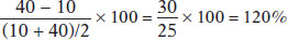
Similarly, the percent increase in her income is

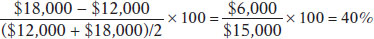
Chelsea’s income elasticity of demand for DVDs is therefore 120%/40% = 3.

2. As the price of margarine rises by 20%, a manufacturer of baked goods increases its quantity of butter demanded by 5%. Calculate the cross-price elasticity of demand between butter and margarine. Are butter and margarine substitutes or complements for this manufacturer?

The cross-price elasticity of demand is 5%/20% = 0.25. Since the cross-price elasticity of demand is positive, the two goods are substitutes.

3. Using the midpoint method, calculate the price elasticity of supply for web-design services when the price per hour rises from $100 to $150 and the number of hours supplied increases from 300,000 hours to 500,000. Is supply elastic, inelastic, or unit-elastic?

By the midpoint method, the percent change in the number of hours of web-design services contracted is

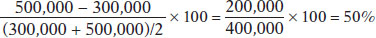
Similarly, the percent change in the price of web-design services is:

The price elasticity of supply is 50%/40% = 1.25. Hence supply is elastic.

Assume the price of corn rises by 20% and this causes suppliers to increase the quantity of corn supplied by 40%.

1. Calculate the price elasticity of supply.

40%/20% = 2

2. In this case, is supply elastic or inelastic?

elastic

3. Draw a correctly labeled graph of a supply curve illustrating the most extreme case of the category of elasticity you found in part b (either perfectly elastic or perfectly inelastic supply).

4. What would likely be true of the availability of inputs for a firm with the supply curve you drew in part c? Explain.

Inputs are readily available and can be shifted into/out of production at low cost.