1.3 20Maximizing Utility

WHAT YOU WILL LEARN
 Why consumers’ general goal is to maximize utility
 Why the principle of diminishing marginal utility applies to the consumption of most goods and services
 How to use marginal analysis to find the optimal consumption bundle
Earlier in this section we learned about principles for rational economic decision making that lead to the best possible outcomes. In this module, we will show how economists analyze the decisions of rational consumers, those who know what they want and make the most of available opportunities. We begin with the concept of utility—
Utility: It’s All About Getting Satisfaction
When analyzing consumer behavior, we’re looking into how people pursue their needs and wants and the subjective feelings that motivate purchases. Yet there is no simple way to measure subjective feelings. How much satisfaction do I get from my third cookie? Is it less or more than the satisfaction you receive from your first cookie? Does it even make sense to ask that question?
Utility is a measure of personal satisfaction.
Luckily, we don’t need to make comparisons between your feelings and mine. An analysis of consumer behavior requires only the assumption that individuals try to maximize some personal measure of the satisfaction gained from consumption. That measure of satisfaction is known as utility, a concept we use to understand behavior but don’t expect to measure in practice.
Utility and Consumption
We can think of consumers as using consumption to “produce” utility, much in the same way that producers use inputs to produce output. As consumers, we do not make explicit calculations of the utility generated by consumption choices, but we must make choices, and we usually base them on at least a rough attempt to achieve greater satisfaction. I can have either soup or salad with my dinner. Which will I enjoy more? I can go to Disney World this year or put the money toward buying a new car. Which will make me happier? These are the types of questions that go into utility maximization.
The concept of utility offers a way to study choices that are made in a more or less rational way.
A util is a hypothetical unit of utility.
How do we measure utility? For the sake of simplicity, it is useful to suppose that we can measure utility in hypothetical units called—
Figure 20-1 illustrates a utility function. It shows the total utility that Cassie, who likes fried clams, gets from an all-
FIGURE20-1Cassie’s Total Utility and Marginal Utility

Cassie’s utility function slopes upward over most of the range shown, but it gets flatter as the number of clams consumed increases. And in this example it eventually turns downward. According to the information in the table in Figure 20-1, nine clams is a clam too many. Adding that additional clam actually makes Cassie worse off: it would lower her total utility. If she’s rational, of course, Cassie will realize that and not consume the ninth clam.
So when Cassie chooses how many clams to consume, she will make this decision by considering the change in her total utility from consuming one more clam. This illustrates the general point: to maximize total utility, consumers must focus on marginal utility.
The Principle of Diminishing Marginal Utility
The marginal utility of a good or service is the change in total utility generated by consuming one additional unit of that good or service.
The marginal utility curve shows how marginal utility depends on the quantity of a good or service consumed.
In addition to showing how Cassie’s total utility depends on the number of clams she consumes, the table in Figure 20-1 also shows the marginal utility generated by consuming each additional clam—

The marginal utility curve slopes downward because each successive clam adds less to total utility than the previous clam. This is reflected in the table: marginal utility falls from a high of 15 utils for the first clam consumed to –1 for the ninth clam consumed. The fact that the ninth clam has negative marginal utility means that consuming it actually reduces total utility. (Restaurants that offer all-
According to the principle of diminishing marginal utility, each successive unit of a good or service consumed adds less to total utility than does the previous unit.
The basic idea behind the principle of diminishing marginal utility is that the additional satisfaction a consumer gets from one more unit of a good or service declines as the amount of that good or service consumed rises. Or, to put it slightly differently, the more of a good or service you consume, the closer you are to being satiated—
The principle of diminishing marginal utility doesn’t always apply, but it does apply in the great majority of cases, enough to serve as a foundation for our analysis of consumer behavior.
Budgets and Optimal Consumption
The principle of diminishing marginal utility explains why most people eventually reach a limit, even at an all-
What do we mean by cost? As always, the fundamental measure of cost is opportunity cost. Because the amount of money a consumer can spend is limited, a decision to consume more of one good is also a decision to consume less of some other good.
Budget Constraints and Budget Lines
Consider Sammy, whose appetite is exclusively for clams and potatoes. (There’s no accounting for tastes.) He has a weekly income of $20 and since, given his appetite, more of either good is better than less, he spends all of it on clams and potatoes. We will assume that clams cost $4 per pound and potatoes cost $2 per pound. What are his possible choices?
Whatever Sammy chooses, we know that the cost of his consumption bundle cannot exceed the amount of money he has to spend. That is,

A budget constraint limits the cost of a consumer’s consumption bundle to no more than the consumer’s income.
A consumer’s consumption possibilities is the set of all consumption bundles that are affordable, given the consumer’s income and prevailing prices.
Consumers always have limited income, which constrains how much they can consume. So the requirement illustrated by Equation 20-
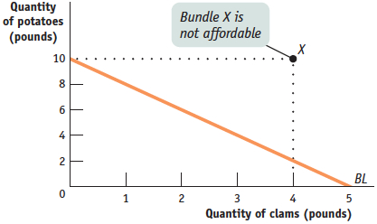
Figure 20-2 shows Sammy’s consumption possibilities. The quantity of clams in his consumption bundle is measured on the horizontal axis and the quantity of potatoes on the vertical axis. The downward-
FIGURE20-2The Budget Line

As an example of one of the points, let’s look at point C, representing 2 pounds of clams and 6 pounds of potatoes, and check whether it satisfies Sammy’s budget constraint. The cost of bundle C is 6 pounds of potatoes × $2 per pound + 2 pounds of clams × $4 per pound = $12 + $8 = $20. So bundle C does indeed satisfy Sammy’s budget constraint: it costs no more than his weekly income of $20. In fact, bundle C costs exactly as much as Sammy’s income. By doing the arithmetic, you can check that all the other points lying on the downward-
A consumer’s budget line shows the consumption bundles available to a consumer who spends all of his or her income.
The downward-
Do we need to consider the other bundles in Sammy’s consumption possibilities, the ones that lie within the shaded region in Figure 20-2 bounded by the budget line? The answer is, for all practical situations, no: as long as Sammy doesn’t get satiated—
Given his $20 per week budget, which point on his budget line will Sammy choose?
The Optimal Consumption Bundle
A consumer’s optimal consumption bundle is the consumption bundle that maximizes the consumer’s total utility given his or her budget constraint.
Because Sammy’s budget constrains him to a consumption bundle somewhere along the budget line, a choice to consume a given quantity of clams also determines his potato consumption, and vice versa. We want to find the consumption bundle—
Table 20-1 shows how much utility Sammy gets from different levels of consumption of clams and potatoes, respectively. According to the table, Sammy has a healthy appetite; the more of either good he consumes, the higher his utility.
20-1
Sammy’s Utility from Clam and Potato Consumption
| Utility from clam consumption | Utility from potato consumption | ||
|---|---|---|---|
| Quantity of clams (pounds) | Utility from clams (utils) | Quantity of potatoes (pounds) | Utility from potatoes (utils) |
| 0 | 0 | 0 | 0 |
| 1 | 15 | 1 | 11.5 |
| 2 | 25 | 2 | 21.4 |
| 3 | 31 | 3 | 29.8 |
| 4 | 34 | 4 | 36.8 |
| 5 | 36 | 5 | 42.5 |
| 6 | 47.0 | ||
| 7 | 50.5 | ||
| 8 | 53.2 | ||
| 9 | 55.2 | ||
| 10 | 56.7 | ||
But because he has a limited budget, he must make a trade-
Table 20-2 shows how his total utility varies for the different consumption bundles along his budget line. Each of six possible consumption bundles, A through F from Figure 20-2, is given in the first column. The second column shows the level of clam consumption corresponding to each choice. The third column shows the utility Sammy gets from consuming those clams. The fourth column shows the quantity of potatoes Sammy can afford given the level of clam consumption; this quantity goes down as his clam consumption goes up because he is sliding down the budget line. The fifth column shows the utility he gets from consuming those potatoes. And the final column shows his total utility. In this example, Sammy’s total utility is the sum of the utility he gets from clams and the utility he gets from potatoes.
20-2
Sammy’s Budget and Total Utility

Figure 20-3 gives a visual representation of the data shown in Table 20-2. Panel (a) shows Sammy’s budget line, to remind us that when he decides to consume more clams he is also deciding to consume fewer potatoes. Panel (b) then shows how his total utility depends on that choice. The horizontal axis in panel (b) has two sets of labels: it shows both the quantity of clams, increasing from left to right, and the quantity of potatoes, increasing from right to left. The reason we can use the same axis to represent consumption of both goods is, of course, that he is constrained by the budget line: the more pounds of clams Sammy consumes, the fewer pounds of potatoes he can afford, and vice versa.
FIGURE20-3Optimal Consumption Bundle


Clearly, the consumption bundle that makes the best of the trade-
As always, we can find the top of the curve by direct observation. We can see from Figure 20-3 that Sammy’s total utility is maximized at point C—that his optimal consumption bundle contains 2 pounds of clams and 6 pounds of potatoes. But we know that we usually gain more insight into “how much” problems when we use marginal analysis. So in the next section we turn to representing and solving the optimal consumption choice problem with marginal analysis.
Spending the Marginal Dollar
As we’ve just seen, we can find Sammy’s optimal consumption choice by finding the total utility he receives from each consumption bundle on his budget line and then choosing the bundle at which total utility is maximized. But we can use marginal analysis instead, turning Sammy’s problem of finding his optimal consumption choice into a “how much” problem.
How do we do this? By thinking about choosing an optimal consumption bundle as a problem of how much to spend on each good. That is, to find the optimal consumption bundle with marginal analysis we ask the question of whether Sammy can make himself better off by spending a little bit more of his income on clams and less on potatoes, or by doing the opposite—
The marginal utility per dollar spent on a good or service is the additional utility from spending one more dollar on that good or service.
Our first step in applying marginal analysis is to ask if Sammy is made better off by spending an additional dollar on either good; and if so, by how much is he better off. To answer this question we must calculate the marginal utility per dollar spent on either clams or potatoes—
Marginal Utility per Dollar
We’ve already introduced the concept of marginal utility, the additional utility a consumer gets from consuming one more unit of a good or service; now let’s see how this concept can be used to derive the related measure of marginal utility per dollar.
Table 20-3 shows how to calculate the marginal utility per dollar spent on clams and potatoes, respectively.
20-3
Sammy’s Marginal Utility per Dollar

In panel (a) of the table, the first column shows different possible amounts of clam consumption. The second column shows the utility Sammy derives from each amount of clam consumption; the third column then shows the marginal utility, the increase in utility Sammy gets from consuming an additional pound of clams. Panel (b) provides the same information for potatoes. The next step is to derive marginal utility per dollar for each good. To do this, we just divide the marginal utility of the good by its price in dollars.
To see why we divide by the price, compare the third and fourth columns of panel (a). Consider what happens if Sammy increases his clam consumption from 2 pounds to 3 pounds. This raises his total utility by 6 utils. But he must spend $4 for that additional pound, so the increase in his utility per additional dollar spent on clams is 6 utils/$4 = 1.5 utils per dollar. Similarly, if he increases his clam consumption from 3 pounds to 4 pounds, his marginal utility is 3 utils but his marginal utility per dollar is 3 utils/$4 = 0.75 utils per dollar.
Notice that because of diminishing marginal utility, Sammy’s marginal utility per pound of clams falls as the quantity of clams he consumes rises. As a result, his marginal utility per dollar spent on clams also falls as the quantity of clams he consumes rises.
So the last column of panel (a) shows how Sammy’s marginal utility per dollar spent on clams depends on the quantity of clams he consumes. Similarly, the last column of panel (b) shows how his marginal utility per dollar spent on potatoes depends on the quantity of potatoes he consumes. Again, marginal utility per dollar spent on each good declines as the quantity of that good consumed rises because of diminishing marginal utility.
We will use the symbols MUC and MUP to represent the marginal utility per pound of clams and potatoes, respectively. And we will use the symbols PC and PP to represent the price of clams (per pound) and the price of potatoes (per pound). Then the marginal utility per dollar spent on clams is MUC/PC and the marginal utility per dollar spent on potatoes is MUP/PP. In general, the additional utility generated from an additional dollar spent on a good is equal to:
Next we’ll see how this concept helps us determine a consumer’s optimal consumption bundle using marginal analysis.
Optimal Consumption
Let’s consider Figure 20-4. As in Figure 20-3, we can measure both the quantity of clams and the quantity of potatoes on the horizontal axis due to the budget constraint. Along the horizontal axis of Figure 20-4—also as in Figure 20-3—the quantity of clams increases as you move from left to right, and the quantity of potatoes increases as you move from right to left. The curve labeled MUC/PC in Figure 20-4 shows Sammy’s marginal utility per dollar spent on clams as derived in Table 20-3. Likewise, the curve labeled MUP/PP shows his marginal utility per dollar spent on potatoes. Notice that the two curves, MUC/PC and MUP/PP, cross at the optimal consumption bundle, point C, consisting of 2 pounds of clams and 6 pounds of potatoes. Moreover, Figure 20-4 illustrates an important feature of Sammy’s optimal consumption bundle: when Sammy consumes 2 pounds of clams and 6 pounds of potatoes, his marginal utility per dollar spent is the same, 2, for both goods. That is, at the optimal consumption bundle, MUC/PC = MUP/PP = 2.
FIGURE20-4Marginal Utility per Dollar

This isn’t an accident. Consider another one of Sammy’s possible consumption bundles—
How do we know this? If Sammy’s marginal utility per dollar spent on clams is higher than his marginal utility per dollar spent on potatoes, he has a simple way to make himself better off while staying within his budget: spend $1 less on potatoes and $1 more on clams. By spending an additional dollar on clams, he adds about 3 utils to his total utility; meanwhile, by spending $1 less on potatoes, he subtracts only about 1 util from his total utility.
Because his marginal utility per dollar spent is higher for clams than for potatoes, reallocating his spending toward clams and away from potatoes would increase his total utility. On the other hand, if his marginal utility per dollar spent on potatoes is higher, he can increase his utility by spending less on clams and more on potatoes. So if Sammy has in fact chosen his optimal consumption bundle, his marginal utility per dollar spent on clams and potatoes must be equal.
This is a general principle, known as the optimal consumption rule: when a consumer maximizes utility in the face of a budget constraint, the marginal utility per dollar spent on each good or service in the consumption bundle is the same. That is, for any two goods C and P, the optimal consumption rule says that at the optimal consumption bundle
The optimal consumption rule says that in order to maximize utility, a consumer must equate the marginal utility per dollar spent on each good and service in the consumption bundle.
It’s easiest to understand this rule using examples in which the consumption bundle contains only two goods, but it applies no matter how many goods or services a consumer buys: the marginal utilities per dollar spent for each and every good or service in the optimal consumption bundle are equal.
The main reason for studying consumer behavior is to look behind the market demand curve. We learned in Section 3 how the substitution effect leads consumers to buy less of a good when its price increases. We used the substitution effect to explain, in general, why the individual demand curve obeys the law of demand. Marginal analysis adds clarity to the utility-
BUYING YOUR WAY OUT OF TEMPTATION

It might seem odd to pay more to get less. But snack food companies have discovered that consumers are indeed willing to pay more for smaller portions, and exploiting this trend is a recipe for success.
Over the last few years, sales of 100-
It’s clear that in this case consumers are making a calculation: the extra utility gained from not having to worry about whether they’ve eaten too much is worth the extra cost. As one shopper said, “They’re pretty expensive, but they’re worth it. It’s individually packaged for the amount I need, so I don’t go overboard.” So it’s clear that consumers aren’t being irrational here. Rather, they’re being entirely rational: in addition to their snack, they’re buying a little hand-
20
Solutions appear at the back of the book.
Check Your Understanding
1. Explain why a rational consumer who has diminishing marginal utility for a good would not consume an additional unit when it generates negative marginal utility, even when that unit is free.
2. In the following two examples, find all the consumption bundles that lie on the consumer’s budget line. Illustrate these consumption possibilities in a diagram, and draw the budget line through them.
-
a. The consumption bundle consists of movie tickets and buckets of popcorn. The price of each ticket is $10.00, the price of each bucket of popcorn is $5.00, and the consumer’s income is $20.00. In your diagram, put movie tickets on the vertical axis and buckets of popcorn on the horizontal axis.
The accompanying table shows the consumer’s consumption possibilities, bundles A through C. These consumption possibilities are plotted in the accompanying diagram, along with the consumer’s budget line.Consumption Bundle Quantity of popcorn (buckets) Quantity of movie tickets A 0 2 B 2 1 C 4 0 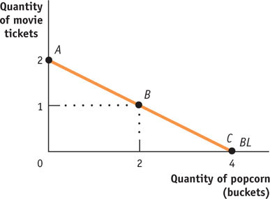
-
b. The consumption bundle consists of underwear and socks. The price of each pair of underwear is $4.00, the price of each pair of socks is $2.00, and the consumer’s income is $12.00. In your diagram, put pairs of socks on the vertical axis and pairs of underwear on the horizontal axis.
The accompanying table shows the consumer’s consumption possibilities, A through D. These consumption possibilities are plotted in the accompanying diagram, along with the consumer’s budget line.Consumption Bundle Quantity of underwear (pairs) Quantity of socks (pairs) A 0 6 B 1 4 C 2 2 D 3 0 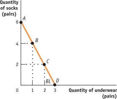
3. In Table 20-3 you can see that the marginal utility per dollar spent on clams and the marginal utility per dollar spent on potatoes are equal when Sammy increases his consumption of clams from 3 pounds to 4 pounds and his consumption of potatoes from 9 pounds to 10 pounds. Explain why this is not Sammy’s optimal consumption bundle. Illustrate your answer using a budget line like the one in Figure 20-3.
Multiple-
Question
1. Generally, each successive unit of a good consumed will cause marginal utility to
| A. |
| B. |
| C. |
| D. |
| E. |
Question
2. Assume there are two goods, good X and good Y. Good X costs $5 and good Y costs $10. If your income is $200, which of the following combinations of good X and good Y is on your budget line?
| A. |
| B. |
| C. |
| D. |
| E. |
Question
3. The optimal consumption rule states that total utility is maximized when all income is spent and
| A. |
| B. |
| C. |
| D. |
| E. |
Question
4. A consumer is spending all of her income and receiving 100 utils from the last unit of good A and 80 utils from the last unit of good B. If the price of good A is $2 and the price of good B is $1, to maximize total utility the consumer should buy
| A. |
| B. |
| C. |
| D. |
| E. |
Question
5. The optimal consumption bundle is always represented by a point
| A. |
| B. |
| C. |
| D. |
| E. |
Critical-
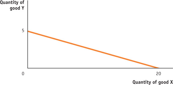
Assume you have an income of $100. The price of good X is $5, and the price of good Y is $20.
1. Draw a correctly labeled budget line with “Quantity of good X” on the horizontal axis and “Quantity of good Y” on the vertical axis. Be sure to correctly label the horizontal and vertical intercepts.
2. With your current consumption bundle, you receive 100 utils from consuming your last unit of good X and 400 utils from consuming your last unit of good Y. Are you maximizing your total utility? Explain.
3. What will happen to the total and marginal utility you receive from consuming good X if you decide to consume another unit of good X? Explain.
THE RIGHT MARGINAL COMPARISON
 Marginal analysis solves “how much” decisions by weighing costs and benefits at the margin: the benefit of doing a little bit more versus the cost of doing a little bit more. But, as we saw in the previous module, the form of the marginal analysis can differ, depending upon whether you are making a production decision or a consumption decision. How do these two forms of marginal analysis differ?
 The form of marginal analysis differs depending upon whether you are making a production decision that maximizes profits or a consumption decision that maximizes utility. In Module 18, Alex’s decision was a production decision because the problem he faced was maximizing the profit from years of schooling. The optimal quantity of years that maximized his profit was found using marginal analysis: at the optimal quantity, the marginal benefit of another year of schooling was equal to its marginal cost. Alex did not face a budget constraint because he could always borrow to finance another year of school.
But if you were to extend the way we solved Alex’s production problem to the consumption problem Sammy faced in Module 20, without any change in form, you might be tempted to say that Sammy’s optimal consumption bundle is the one at which the marginal utility of clams is equal to the marginal utility of potatoes, or that the marginal utility of clams was equal to the price of clams. But both of those statements would be wrong because they don’t properly account for the budget constraint and the fact that consuming more of one good requires consuming less of another. In a consumption decision, your objective is to maximize the utility that your limited budget can deliver. And the right way to find the optimal consumption bundle is to set the marginal utility per dollar equal for each good in the consumption bundle. When this condition is satisfied, the “bang per buck” is the same across all the goods and services you consume. Only then is there no way to rearrange your consumption and get more utility from your budget.
To learn more, reread “Spending the Marginal Dollar,” on pages 216–
