1.1 21The Production Function

WHAT YOU WILL LEARN
 The importance of the firm’s production function, the relationship between the quantity of inputs and the quantity of output
 Why production is often subject to diminishing returns to inputs
The Production Function
A production function is the relationship between the quantity of inputs a firm uses and the quantity of output it produces.
A firm produces goods or services for sale. To do this, it must transform inputs into output. The quantity of output a firm produces depends on the quantity of inputs; this relationship is known as the firm’s production function. As we’ll see, a firm’s production function underlies its cost curves. As a first step, let’s look at the characteristics of a hypothetical production function.
Inputs and Output
To understand the concept of a production function, let’s consider a farm that we assume, for the sake of simplicity, produces only one output, wheat, and uses only two inputs, land and labor. This particular farm is owned by a couple named George and Martha. They hire workers to do the actual physical labor on the farm. Moreover, we will assume that all potential workers are of the same quality—
A fixed input is an input whose quantity is fixed for a period of time and cannot be varied.
A variable input is an input whose quantity the firm can vary at any time.
George and Martha’s farm sits on 10 acres of land; no more acres are available to them, and they are currently unable to either increase or decrease the size of their farm by selling, buying, or leasing acreage. Land here is what economists call a fixed input—an input whose quantity is fixed for a period of time and cannot be varied. George and Martha are, however, free to decide how many workers to hire. The labor provided by these workers is called a variable input—an input whose quantity the firm can vary at any time.
The long run is the time period in which all inputs can be varied.
The short run is the time period in which at least one input is fixed.
In reality, whether or not the quantity of an input is really fixed depends on the time horizon. In the long run—that is, given that a long enough period of time has elapsed—
George and Martha know that the quantity of wheat they produce depends on the number of workers they hire. Using modern farming techniques, one worker can cultivate the 10-
The total product curve shows how the quantity of output depends on the quantity of the variable input, for a given quantity of the fixed input.
The relationship between the quantity of labor and the quantity of output, for a given amount of the fixed input, constitutes the farm’s production function. The production function for George and Martha’s farm, where land is the fixed input and labor is the variable input, is shown in the first two columns of the table in Figure 21-1; the diagram there depicts the same information graphically. The curve in Figure 21-1 shows how the quantity of output depends on the quantity of the variable input for a given quantity of the fixed input; it is called the farm’s total product curve. The physical quantity of output, bushels of wheat, is measured on the vertical axis; the quantity of the variable input, labor (that is, the number of workers employed), is measured on the horizontal axis. The total product curve here slopes upward, reflecting the fact that more bushels of wheat are produced as more workers are employed.
FIGURE21-1Production Function and Total Product Curve for George and Martha’s Farm

The marginal product of an input is the additional quantity of output produced by using one more unit of that input.
Although the total product curve in Figure 21-1 slopes upward along its entire length, the slope isn’t constant: as you move up the curve to the right, it flattens out. To understand this changing slope, look at the third column of the table in Figure 21-1, which shows the change in the quantity of output generated by adding one more worker. That is, it shows the marginal product of labor, or MPL: the additional quantity of output from using one more unit of labor (one more worker).
In this example, we have data at intervals of 1 worker—

or

Note that Δ, the Greek uppercase delta, represents the change in a variable.
Now we can explain the significance of the slope of the total product curve: it is equal to the marginal product of labor. The slope of a line is equal to “rise” over “run.” This implies that the slope of the total product curve is the change in the quantity of output (the “rise”) divided by the change in the quantity of labor (the “run”). And this, as we can see from Equation 21-
In this example, the marginal product of labor steadily declines as more workers are hired—
Figure 21-2 shows how the marginal product of labor depends on the number of workers employed on the farm. The marginal product of labor, MPL, is measured on the vertical axis in units of physical output—
FIGURE21-2Marginal Product of Labor Curve for George and Martha’s Farm

There are diminishing returns to an input when an increase in the quantity of that input, holding the levels of all other inputs fixed, leads to a decline in the marginal product of that input.
In this example the marginal product of labor falls as the number of workers increases. That is, there are diminishing returns to labor on George and Martha’s farm. In general, there are diminishing returns to an input when an increase in the quantity of that input, holding the quantity of all other inputs fixed, reduces that input’s marginal product. Due to diminishing returns to labor, the MPL curve is negatively sloped.
To grasp why diminishing returns can occur, think about what happens as George and Martha add more and more workers without increasing the number of acres. As the number of workers increases, the land is farmed more intensively and the number of bushels increases. But each additional worker is working with a smaller share of the 10 acres—
The crucial point to emphasize about diminishing returns is that, like many propositions in economics, it is an “other things equal” proposition: each successive unit of an input will raise production by less than the last if the quantity of all other inputs is held fixed.

What would happen if the levels of other inputs were allowed to change? You can see the answer illustrated in Figure 21-3. Panel (a) shows two total product curves, TP10 and TP20. TP10 is the farm’s total product curve when its total area is 10 acres (the same curve as in Figure 21-1). TP20 is the total product curve when the farm’s area has increased to 20 acres. Except when 0 workers are employed, TP20 lies everywhere above TP10 because with more acres available, any given number of workers produces more output. Panel (b) shows the corresponding marginal product of labor curves. MPL10 is the marginal product of labor curve given 10 acres to cultivate (the same curve as in Figure 21-2), and MPL20 is the marginal product of labor curve given 20 acres. Both curves slope downward because, in each case, the amount of land is fixed, although at different levels. But MPL20 lies everywhere above MPL10, reflecting the fact that the marginal product of the same worker is higher when he or she has more of the fixed input to work with.
FIGURE21-3Total Product, Marginal Product, and the Fixed Input

Figure 21-3 demonstrates a general result: the position of the total product curve depends on the quantities of other inputs. If you change the quantities of the other inputs, both the total product curve and the marginal product curve of the remaining input will shift.
THE MYTHICAL MAN-MONTH
The concept of diminishing returns to an input was first formulated by economists during the late eighteenth century. These economists, notably including Thomas Malthus, drew their inspiration from agricultural examples. Although still valid, examples drawn from agriculture can seem somewhat musty and old-
However, the idea of diminishing returns to an input applies with equal force to the most modern of economic activities—
The chapter that gave its title to the book is basically about diminishing returns to labor in the writing of software. Brooks observed that multiplying the number of programmers assigned to a project did not produce a proportionate reduction in the time it took to get the program written. A project that could be done by one programmer in 12 months could not be done by 12 programmers in one month. The “mythical man-
The argument of The Mythical Man-
FIGURE21-4Mythical Man-Month

In other words, programming is subject to diminishing returns so severe that at some point more programmers actually have negative marginal product. The source of the diminishing returns lies in the nature of the production function for a programming project: each programmer must coordinate his or her work with that of all the other programmers on the project, leading to each person spending more time communicating with others—
21
Solutions appear at the back of the book.
Check Your Understanding
1. Bernie’s ice-
-
a. What is the fixed input? What is the variable input?
The fixed input is the 10-ton machine and the variable input is electricity. -
b. Construct a table showing the marginal product of the variable input. Does it show diminishing returns?
As you can see from the declining numbers in the third column of the accompanying table, electricity does indeed exhibit diminishing returns: the marginal product of each additional kilowatt of electricity is less than that of the previous kilowatt.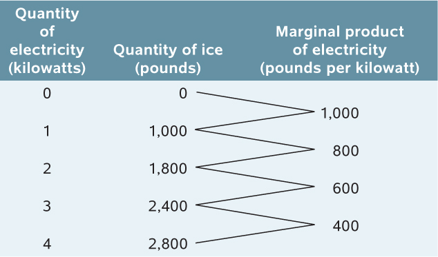
-
c. Suppose a 50% increase in the size of the fixed input increases output by 100% for any given amount of the variable input. What is the fixed input now? Construct a table showing the quantity of output and the marginal product in this case.
| Quantity of electricity (kilowatts) | Quantity of ice (pounds) |
|---|---|
| 0 | 0 |
| 1 | 1,000 |
| 2 | 1,800 |
| 3 | 2,400 |
| 4 | 2,800 |
A 50% increase in the size of the fixed input means that Bernie now has a 15-ton machine, so the fixed input is now the 15-ton machine. Since it generates a 100% increase in output for any given amount of electricity, the quantity of output and the marginal product are now as shown in the accompanying table.
Multiple-
Question
1. A production function shows the relationship between inputs and
| A. |
| B. |
| C. |
| D. |
| E. |
Question
2. Which of the following defines the short run?
| A. |
| B. |
| C. |
| D. |
| E. |
Question
3. The slope of the total product curve is also known as
| A. |
| B. |
| C. |
| D. |
| E. |
Question
4. Diminishing returns to an input means that as a firm continues to produce, the total product curve will have what kind of slope?
| A. |
| B. |
| C. |
| D. |
| E. |
Question
5. Historically, the limits imposed by diminishing returns have been alleviated by
| A. |
| B. |
| C. |
| D. |
| E. |
Critical-
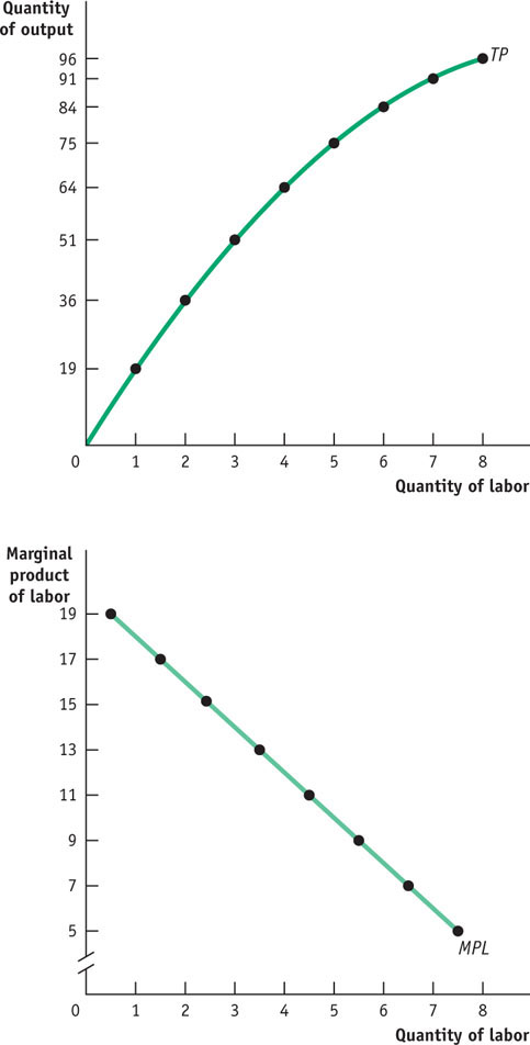
Use the data in the table below to graph the production function and the marginal product of labor. Do the data illustrate diminishing returns to labor? Explain.
| Quantity of labor | Quantity of output |
|---|---|
| L | Q |
| 0 | 0 |
| 1 | 19 |
| 2 | 36 |
| 3 | 51 |
| 4 | 64 |
| 5 | 75 |
| 6 | 84 |
| 7 | 91 |
| 8 | 96 |
WHAT ARE THE RIGHT UNITS TO USE?
 The marginal product of labor (or any other input) is defined as the increase in the quantity of output when you increase the quantity of that input by one unit. But when we say a “unit” of labor, do we mean an additional hour of labor, an additional week, or a person-
 It doesn’t matter, as long as you are consistent. whatever units you use, always be careful that you use the same units throughout your analysis of any problem. One common source of error in economics is getting units confused—
To learn more, review the definition of marginal product of labor.
