1.2 25Perfect Competition
WHAT YOU WILL LEARN
 How a price-
taking firm determines its profit- maximizing quantity of output  How to assess whether or not a competitive firm is profitable
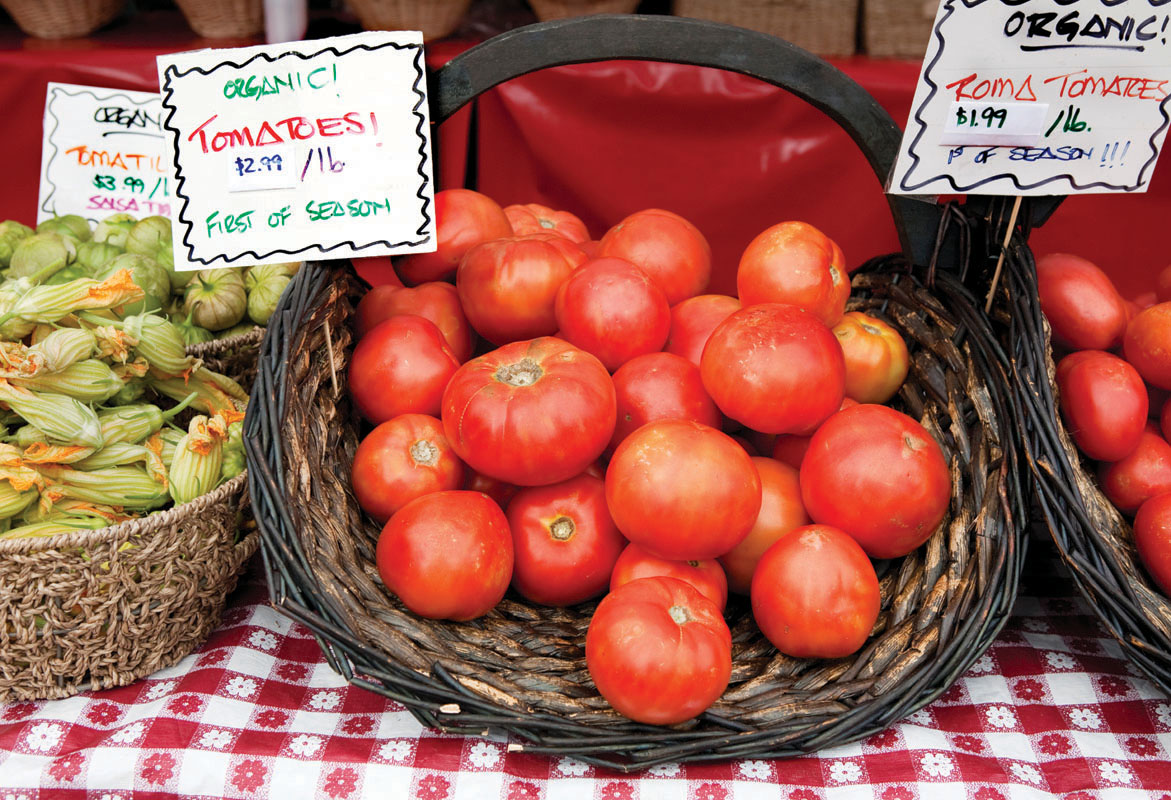
Recall the example of the market for organic tomatoes from the previous module. There, Yves and Zoe run organic tomato farms. But many other organic tomato farmers sell their output to the same grocery store chains. Since organic tomatoes are a standardized product, consumers don’t care which farmer produces the organic tomatoes they buy. And because so many farmers sell organic tomatoes, no individual farmer has a large market share, which means that no individual farmer can have a measurable effect on market prices. These farmers are price-
Production and Profits
Let’s now consider Jennifer and Jason, who, like Yves and Zoe, run an organic tomato farm. Suppose that the market price of organic tomatoes is $18 per bushel and that Jennifer and Jason can sell as many as they would like at that price. We can use the data in Table 25-1 to find their profit-
25-1
Profit for Jennifer and Jason’s Farm When the Market Price Is $18

The first column shows the quantity of output in bushels, and the second column shows Jennifer and Jason’s total revenue from their output: the market value of their output. Total revenue, TR, is equal to the market price multiplied by the quantity of output:

In this example, total revenue is equal to $18 per bushel times the quantity of output in bushels.
The third column of Table 25-1 shows Jennifer and Jason’s total cost, TC. The fourth column shows their profit, equal to total revenue minus total cost:

As indicated by the numbers in the table, profit is maximized at an output of five bushels, where profit is equal to $18. But we can gain more insight into the profit-
Using Marginal Analysis to Choose the Profit-Maximizing Quantity of Output
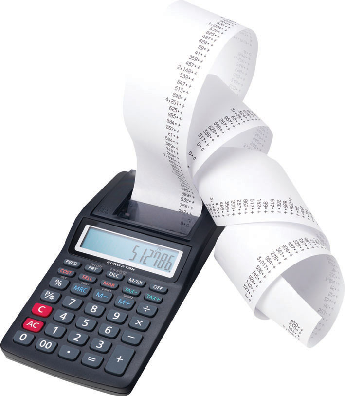
Marginal revenue is the change in total revenue generated by an additional unit of output.
Recall from Module 18 the profit-
or
MR = ΔTR/ΔQ
In this equation, the Greek uppercase delta (the triangular symbol) represents the change in a variable.
The optimal output rule says that profit is maximized by producing the quantity of output at which the marginal revenue of the last unit produced is equal to its marginal cost
So Jennifer and Jason maximize their profit by producing bushels up to the point at which marginal revenue is equal to marginal cost. We can summarize this result as the producer’s optimal output rule, which states that profit is maximized by producing the quantity at which the marginal revenue of the last unit produced is equal to its marginal cost. That is, MR = MC at the optimal quantity of output.
Note that there may not be any particular quantity at which marginal revenue exactly equals marginal cost. In this case the producer should produce until one more unit would cause marginal benefit to fall below marginal cost. As a common simplification, we can think of marginal cost as rising steadily, rather than jumping from one level at one quantity to a different level at the next quantity. This ensures that marginal cost will equal marginal revenue at some quantity. We will now employ this simplified approach.
Consider Table 25-2, which provides cost and revenue data for Jennifer and Jason’s farm. The second column contains the farm’s total cost of output. The third column shows their marginal cost. Notice that, in this example, marginal cost initially falls as output rises but then begins to increase, so that the marginal cost curve has a “swoosh” shape. (Later you will see that this shape has important implications for short-
25-2
Short-Run Costs for Jennifer and Jason's Farm

The fourth column contains the farm’s marginal revenue, which has an important feature: Jennifer and Jason’s marginal revenue is assumed to be constant at $18 for every output level. The fifth and final column shows the calculation of the net gain per bushel of tomatoes, which is equal to marginal revenue minus marginal cost. As you can see, it is positive for the first through fifth bushels; producing each of these bushels raises Jennifer and Jason’s profit. For the sixth and seventh bushels, however, net gain is negative: producing them would decrease, not increase, profit. (You can verify this by reexamining Table 25-1.) So five bushels are Jennifer and Jason’s profit-
This example, in fact, illustrates an application of the optimal output rule to the particular case of a price-
According to the price-
In fact, the price-
A price-
Figure 25-1 shows that Jennifer and Jason’s profit-
FIGURE25-1The Firm’s Profit-Maximizing Quantity of Output

The marginal revenue curve shows how marginal revenue varies as output varies.
We plot the marginal cost of increasing output from one to two bushels halfway between one and two, and so on. The horizontal line at $18 is Jennifer and Jason’s marginal revenue curve, which shows how marginal revenue varies as output varies. Note that marginal revenue stays the same regardless of how much Jennifer and Jason sell because we have assumed marginal revenue is constant.
Does this mean that the firm’s production decision can be entirely summed up as “produce up to the point where the marginal cost of production is equal to the price”? No, not quite. Before applying the price-
To understand why the first step in the production decision involves an “either–
When Is Production Profitable?
Remember that firms make their production decisions with the goal of maximizing economic profit—a measure based on the opportunity cost of resources used by the firm. In the calculation of economic profit, a firm’s total cost incorporates the implicit cost—the benefits forgone in the next best use of the firm’s resources—
In contrast, accounting profit is profit calculated using only the explicit costs incurred by the firm. This means that economic profit incorporates all of the opportunity cost of resources owned by the firm and used in the production of output, while accounting profit does not.
A firm may make positive accounting profit while making zero or even negative economic profit. It’s important to understand that a firm’s decisions of how much to produce, and whether or not to stay in business, should be based on economic profit, not accounting profit.
So we will assume, as usual, that the cost numbers given in Table 25-1 include all costs, implicit as well as explicit. What determines whether Jennifer and Jason’s farm earns a profit or generates a loss? This depends on the market price of tomatoes—
In Table 25-3 we calculate short-
25-3
Short-
| Quantity of tomatoes Q (bushels) |
Variable cost VC |
Total cost TC |
Short- AVC = VC/Q |
Short- ATC = TC/Q |
|---|---|---|---|---|
| 1 | $16.00 | $30.00 | $16.00 | $30.00 |
| 2 | 22.00 | 36.00 | 11.00 | 18.00 |
| 3 | 30.00 | 44.00 | 10.00 | 14.67 |
| 4 | 42.00 | 56.00 | 10.50 | 14.00 |
| 5 | 58.00 | 72.00 | 11.60 | 14.40 |
| 6 | 78.00 | 92.00 | 13.00 | 15.33 |
| 7 | 102.00 | 116.00 | 14.57 | 16.57 |
FIGURE25-2Costs and Production in the Short Run

To see how these curves can be used to decide whether production is profitable or unprofitable, recall that profit is equal to total revenue minus total cost, TR − TC. This means:
- If the firm produces a quantity at which TR > TC, the firm is profitable.
- If the firm produces a quantity at which TR = TC, the firm earns neither a profit nor a loss—
it breaks even. - If the firm produces a quantity at which TR <TC, the firm incurs a loss.
We can also express this idea in terms of revenue and cost per unit of output. If we divide profit by the number of units of output, Q, we obtain the following expression for profit per unit of output:

TR/Q is average revenue, which is the market price. TC/Q is average total cost. So a firm is profitable if the market price for its product is more than the average total cost of the quantity the firm produces; a firm experiences losses if the market price is less than the average total cost of the quantity the firm produces. This means:
- If the firm produces a quantity at which P > ATC, the firm is profitable.
- If the firm produces a quantity at which P = ATC, the firm earns neither a profit nor a loss—
it breaks even. - If the firm produces a quantity at which P < ATC, the firm incurs a loss.
In summary, in the short run a firm will maximize profit by producing the quantity of output at which MC = MR. A perfectly competitive firm is a price-
25
Solutions appear at the back of the book.
Check Your Understanding
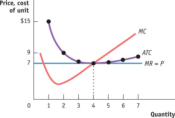
1. Refer to the graph provided to answer the questions that follow.
-
a. At what level of output does the firm maximize profit? Explain how you know.
The firm maximizes profit at a quantity of 4, because it is at that quantity that MC = MR. -
b. At the profit-
maximizing quantity of output, is the firm profitable, does it just break even, or does it earn a loss? Explain. At a quantity of 4 the firm just breaks even. This is because at a quantity of 4, P = ATC, so the amount the firm takes in for each unit—the price—exactly equals the average total cost per unit.
2. If a firm has a total cost of $500 at a quantity of 50 units, and it is at that quantity that average total cost is minimized for the firm, what is the lowest price that would allow the firm to break even? Explain.
Multiple-
Question
1. A perfectly competitive firm will maximize profit at the quantity at which the firm’s marginal revenue equals
| A. |
| B. |
| C. |
| D. |
| E. |
Question
2. Which of the following is correct for a perfectly competitive firm?
I. The marginal revenue curve is the demand curve.
II. The firm maximizes profit when price equals marginal cost.
III. The demand curve is horizontal.
| A. |
| B. |
| C. |
| D. |
| E. |
Question
3. A firm is profitable if
| A. |
| B. |
| C. |
| D. |
| E. |
Question
4. If a firm has a total cost of $200, its profit-
| A. |
| B. |
| C. |
| D. |
| E. |
Question
5. What is the firm’s profit if the price of its product is $5 and it produces 500 units of output at a total cost of $1,000?
| A. |
| B. |
| C. |
| D. |
| E. |
Critical-
The table provided presents the short-
1. calculate the firm’s marginal cost at each quantity.
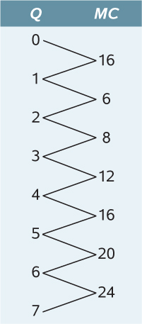
2. determine the firm’s profit-
3. calculate the firm’s profit at the profit-
|
Quantity of tomatoes Q (bushels) |
Variable cost VC |
Total cost TC |
|---|---|---|
| 0 | $0 | $14 |
| 1 | 16 | 30 |
| 2 | 22 | 36 |
| 3 | 30 | 44 |
| 4 | 42 | 56 |
| 5 | 58 | 72 |
| 6 | 78 | 92 |
| 7 | 102 | 116 |
WHAT’S A FIRM TO DO?
 The optimal output rule says that to maximize profit, a firm should produce the quantity at which marginal revenue is equal to marginal cost. But what should a firm do if there is no output level at which marginal revenue equals marginal cost?
![]() In this case, a firm would produce the largest quantity for which marginal revenue exceeds marginal cost. This is the case in Table 25-2 at an output of 5 bushels. However, a simpler version of the optimal output rule applies when production involves much larger numbers, such as hundreds or thousands of units. In such cases, marginal cost comes in small increments, and there is always a level of output at which marginal cost almost exactly equals marginal revenue.
In this case, a firm would produce the largest quantity for which marginal revenue exceeds marginal cost. This is the case in Table 25-2 at an output of 5 bushels. However, a simpler version of the optimal output rule applies when production involves much larger numbers, such as hundreds or thousands of units. In such cases, marginal cost comes in small increments, and there is always a level of output at which marginal cost almost exactly equals marginal revenue.
To learn more, see pages 271–
