1.4 Module 27: Long-Run Outcomes in Perfect Competition

© George Kroll | Dreamstime.com

Up to this point we have been discussing the perfectly competitive firm’s short-run situation—whether to produce or not, and if so, whether the firm earns a positive profit, breaks even, or takes a loss. In this module, we look at the long-run situation in a perfectly competitive market. We will see that perfect competition leads to some interesting and desirable market outcomes. In upcoming sections, we will contrast these outcomes with the outcomes in monopolistic and imperfectly competitive markets.

The Industry Supply Curve

Why will an increase in the demand for organic tomatoes lead to a large price increase at first but a much smaller increase in the long run? The answer lies in the behavior of the industry supply curve—the relationship between the price and the total output of an industry as a whole. The industry supply curve is what we referred to in earlier modules as the supply curve or the market supply curve. But here we take some extra care to distinguish between the individual supply curve of a single firm and the supply curve of the industry as a whole.

As you might guess from the previous module, the industry supply curve must be analyzed in somewhat different ways for the short run and the long run. Let’s start with the short run.

The Short-Run Industry Supply Curve

Recall that in the short run the number of firms in an industry is fixed—there is no entry or exit. And you may also remember from Section 2 that the market supply curve is the horizontal sum of the individual supply curves of all firms—you find it by summing the total output across all suppliers at every given price. We will do that exercise here under the assumption that all the firms are alike—an assumption that makes the derivation particularly simple. So let’s assume that there are 100 organic tomato farms, each with the same costs as Jennifer and Jason’s farm.

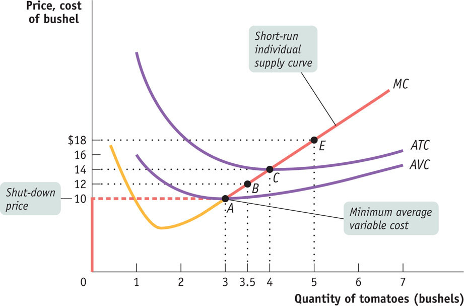
Each of these 100 farms will have an individual short-run supply curve like the one in Figure 26-2 from the previous module, which appears again here, as Figure 27-1 for your convenience.

When the market price equals or exceeds Jennifer and Jason’s shut-down price of $10, the minimum average variable cost indicated by point A, they will produce the output quantity at which marginal cost is equal to price. So at any price equal to or above the minimum average variable cost, the short-run individual supply curve is the firm’s marginal cost curve; this corresponds to the upward-sloping segment of the individual supply curve. When market price falls below minimum average variable cost, the firm ceases operation in the short run. This corresponds to the vertical segment of the individual supply curve along the vertical axis.

At a price below $10, no farms will produce. At a price of more than $10, each farm will produce the quantity of output at which its marginal cost is equal to the market price. As you can see from Figure 27-1, this will lead each farm to produce 4 bushels if the price is $14 per bushel, 5 bushels if the price is $18, and so on.

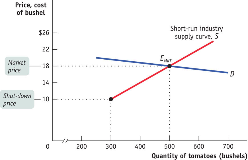
So if there are 100 organic tomato farms and the price of organic tomatoes is $18 per bushel, the industry as a whole will produce 500 bushels, corresponding to 100 farms × 5 bushels per farm. The result is the short-run industry supply curve, shown as S in Figure 27-2. This curve shows the quantity that producers will supply at each price, taking the number of farms as given.

The short-run industry supply curve, S, is the industry supply curve taking the number of producers—here, 100—as given. It is generated by adding together the individual supply curves of the 100 producers. Below the shut-down price of $10, no producer wants to produce in the short run. Above $10, the short-run industry supply curve slopes upward, as each producer increases output as price increases. It intersects the demand curve, D, at point E_MKT, the point of short-run market equilibrium, corresponding to a market price of $18 and a quantity of 500 bushels.

The market demand curve, labeled D in Figure 27-2, crosses the short-run industry supply curve at E_MKT, corresponding to a price of $18 and a quantity of 500 bushels. Point E_MKT is a short-run market equilibrium: the quantity supplied equals the quantity demanded, taking the number of farms as given. But the long run may look quite different because in the long run farms may enter or exit the industry.

The Long-Run Industry Supply Curve

Suppose that in addition to the 100 farms currently in the organic tomato business, there are many other potential organic tomato farms. Suppose also that each of these potential farms would have the same cost curves as existing farms, like the one owned by Jennifer and Jason, upon entering the industry.

When will additional farms enter the industry? Whenever existing farms are making a profit—that is, whenever the market price is above the break-even price of $14 per bushel, the minimum average total cost of production. For example, at a price of $18 per bushel, new farms will enter the industry.

What will happen as additional farms enter the industry? Clearly, the quantity supplied at any given price will increase. The short-run industry supply curve will shift to the right. This will, in turn, alter the market equilibrium and result in a lower market price. Existing farms will respond to the lower market price by reducing their output, but the total industry output will increase because of the larger number of farms in the industry.

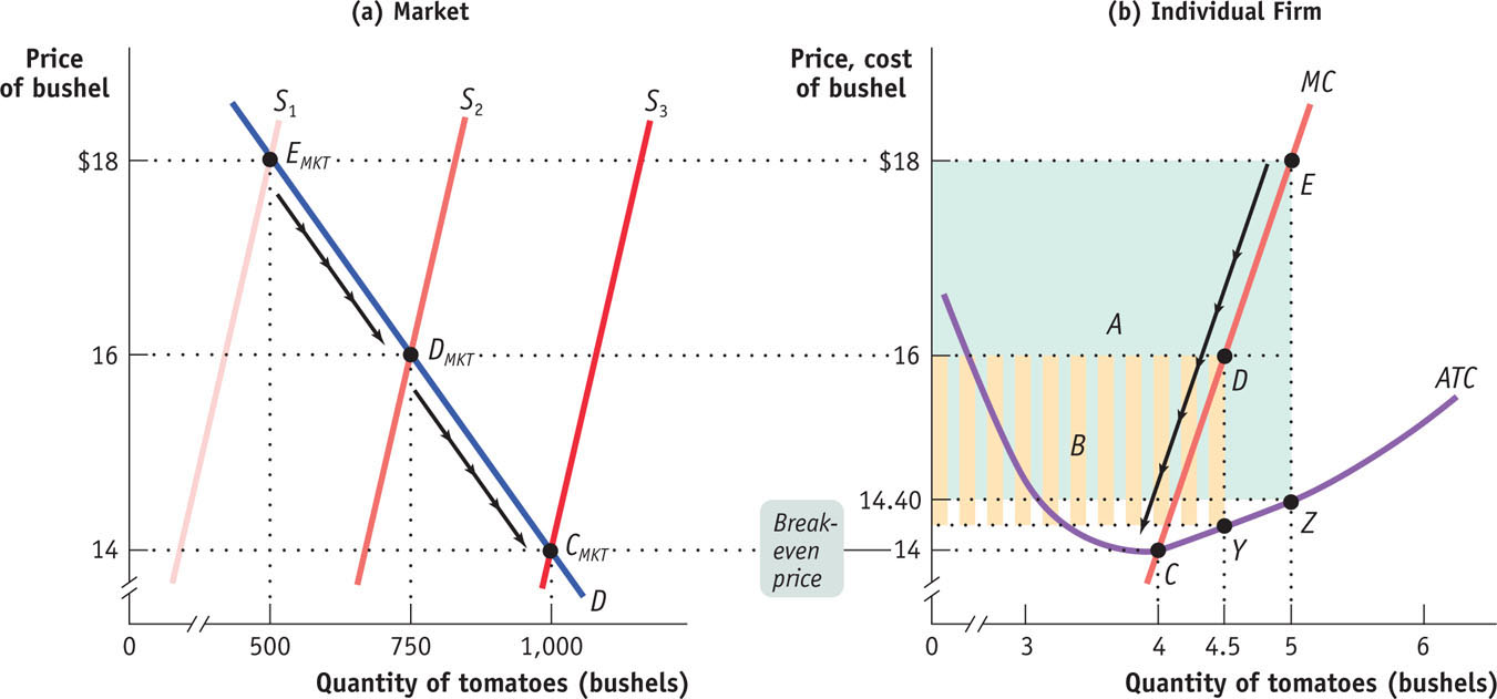
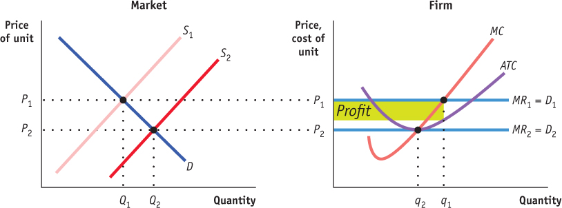
Figure 27-3 illustrates the effects of this chain of events on an existing farm and on the market; panel (a) shows how the market responds to entry, and panel (b) shows how an individual existing farm responds to entry. (Note that these two graphs have been rescaled in comparison to Figures 27-1 and 27-2 to better illustrate how profit changes in response to price.) In panel (a), S₁ is the initial short-run industry supply curve, based on the existence of 100 producers. The initial short-run market equilibrium is at E_MKT, with an equilibrium market price of $18 and a quantity of 500 bushels. At this price existing farms are profitable, which is reflected in panel (b): an existing farm makes a total profit represented by the green shaded rectangle labeled A when the market price is $18.

Point E_MKT of panel (a) shows the initial short-run market equilibrium. Each of the 100 existing producers makes an economic profit, illustrated in panel (b) by the green rectangle labeled A, the profit of an existing firm. Profits induce entry by additional producers, shifting the short-run industry supply curve outward from S₁ to S₂ in panel (a), resulting in a new short-run equilibrium at point D_MKT, at a lower market price of $16 and higher industry output. Existing firms reduce output and profit falls to the area given by the striped rectangle labeled B in panel (b). Entry continues to shift out the short-run industry supply curve, as price falls and industry output increases yet again. Entry ceases at point C_MKT on supply curve S₃ in panel (a). Here market price is equal to the break-even price; existing producers make zero economic profits and there is no incentive for entry or exit. Therefore C_MKT is also a long-run market equilibrium.

These profits will induce new producers to enter the industry, shifting the short-run industry supply curve to the right. For example, the short-run industry supply curve when the number of farms has increased to 167 is S₂. Corresponding to this supply curve is a new short-run market equilibrium labeled D_MKT, with a market price of $16 and a quantity of 750 bushels. At $16, each farm produces 4.5 bushels, so that industry output is 167 × 4.5 = 750 bushels (rounded). From panel (b) you can see the effect of the entry of 67 new farms on an existing farm: the fall in price causes it to reduce its output, and its profit falls to the area represented by the striped rectangle labeled B.

Although diminished, the profit of existing farms at D_MKT means that entry will continue and the number of farms will continue to rise. If the number of farms rises to 250, the short-run industry supply curve shifts out again to S₃, and the market equilibrium is at C_MKT, with a quantity supplied and demanded of 1,000 bushels and a market price of $14 per bushel.

Like E_MKT and D_MKT, C_MKT is a short-run equilibrium. But it is also something more. Because the price of $14 is each farm’s break-even price, an existing producer makes zero economic profit—neither a profit nor a loss, earning only the opportunity cost of the resources used in production—when producing its profit-maximizing output of 4 bushels. At this price there is no incentive either for potential producers to enter or for existing producers to exit the industry. So C_MKT corresponds to a long-run market equilibrium—a situation in which the quantity supplied equals the quantity demanded, given that sufficient time has elapsed for producers to either enter or exit the industry. In a long-run market equilibrium, all existing and potential producers have fully adjusted to their optimal long-run choices; as a result, no producer has an incentive to either enter or exit the industry.

!world_eia!BALING IN, BAILING OUT

“King Cotton is back,” proclaimed a 2010 article in the Los Angeles Times, describing a cotton boom that had “turned great swaths of Central California a snowy white during harvest season.” Cotton prices were soaring: they more than tripled between early 2010 and early 2011. And farmers responded by planting more cotton.

King Cotton’s reign will inevitably end as new producers enter the market and bring prices down.

PhotoAlto/Superstock27UN02

What was behind the price rise? As we learned in Section 2, it was partly caused by temporary factors, notably severe floods in Pakistan that destroyed much of that nation’s cotton crop. But there was also a big rise in demand, especially from China, whose burgeoning textile and clothing industries demanded ever more raw cotton to weave into cloth. And all indications were that higher demand was here to stay.

So is cotton farming going to be a highly profitable business from now on? The answer is no, because when an industry becomes highly profitable, it draws in new producers, and that brings prices down. And the cotton industry was following the standard script.

For it wasn’t just the Central Valley of California that had turned “snowy white.” Farmers around the world were moving into cotton growing. “This summer, cotton will stretch from Queensland through northern NSW [New South Wales] all the way down to the Murrumbidgee valley in southern NSW,” declared an Australian report.

And by 2012, the entry of all these new producers had a big effect. By the summer of 2012, cotton prices were only about a third of their peak in early 2011. It was clear that the cotton boom had reached its limit—and that at some point in the not too distant future some of the farmers who had rushed into the industry would leave it again.

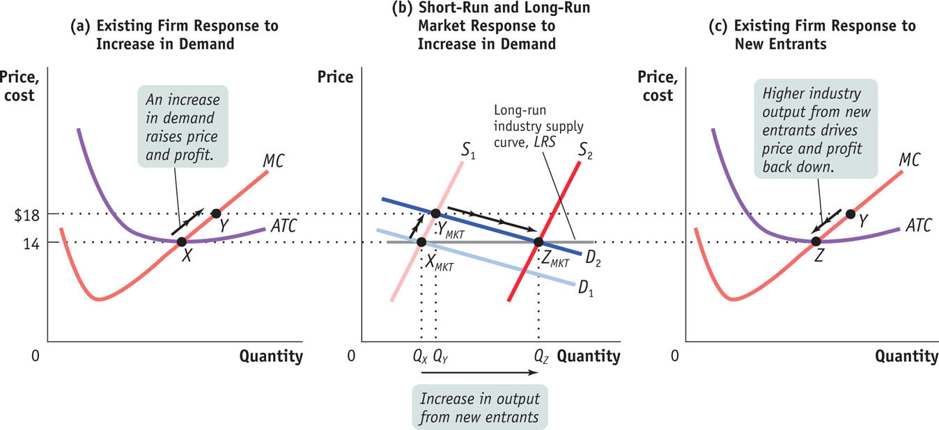
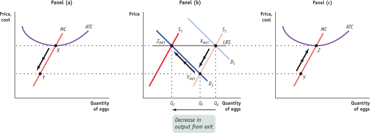
To explore further the difference between short-run and long-run equilibrium, consider the effect of an increase in demand on an industry with free entry that is initially in long-run equilibrium. Panel (b) in Figure 27-4 shows the market adjustment; panels (a) and (c) show how an existing individual firm behaves during the process.

Panel (b) shows how an industry adjusts in the short and long run to an increase in demand; panels (a) and (c) show the corresponding adjustments by an existing firm. Initially the market is at point X_MKT in panel (b), a short-run and long-run equilibrium at a price of $14 and industry output of Q_X. An existing firm makes zero economic profit, operating at point X in panel (a) at minimum average total cost. Demand increases as D₁ shifts rightward to D₂, in panel (b), raising the market price to $18. Existing firms increase their output, and industry output moves along the short-run industry supply curve S₁ to a short-run equilibrium at Y_MKT. Correspondingly, the existing firm in panel (a) moves from point X to point Y. But at a price of $18 existing firms are profitable. As shown in panel (b), in the long run new entrants arrive and the short-run industry supply curve shifts rightward, from S₁ to S₂. There is a new equilibrium at point Z_MKT, at a lower price of $14 and higher industry output of Q_Z. An existing firm responds by moving from Y to Z in panel (c), returning to its initial output level and zero economic profit. Production by new entrants accounts for the total increase in industry output, Q_Z − Q_X. Like X_MKT, Z_MKT is also a short-run and long-run equilibrium: with existing firms earning zero economic profit, there is no incentive for any firms to enter or exit the industry. The horizontal line passing through X_MKT and Z_MKT, LRS, is the long-run industry supply curve: at the break-even price of $14, producers will produce any amount that consumers demand in the long run.

In panel (b) of Figure 27-4, D₁ is the initial demand curve and S₁ is the initial short-run industry supply curve. Their intersection at point X_MKT is both a short-run and a long-run market equilibrium because the equilibrium price of $14 leads to zero economic profit—and therefore neither entry nor exit. It corresponds to point X in panel (a), where an individual existing firm is operating at the minimum of its average total cost curve.

Now suppose that the demand curve shifts out for some reason to D₂. As shown in panel (b), in the short run, industry output moves along the short-run industry supply curve, S₁, to the new short-run market equilibrium at Y_MKT, the intersection of S₁ and D₂. The market price rises to $18 per bushel, and industry output increases from Q_X to Q_Y. This corresponds to an existing firm’s movement from X to Y in panel (a) as the firm increases its output in response to the rise in the market price.

But we know that Y_MKT is not a long-run equilibrium because $18 is higher than minimum average total cost, so existing firms are making economic profits. This will lead additional firms to enter the industry. Over time entry will cause the short-run industry supply curve to shift to the right. In the long run, the short-run industry supply curve will have shifted out to S₂, and the equilibrium will be at Z_MKT—with the price falling back to $14 per bushel and industry output increasing yet again, from Q_Y to Q_Z. Like X_MKT before the increase in demand, Z_MKT is both a short-run and a long-run market equilibrium.

The effect of entry on an existing firm is illustrated in panel (c), in the movement from Y to Z along the firm’s individual supply curve. The firm reduces its output in response to the fall in the market price, ultimately arriving back at its original output quantity, corresponding to the minimum of its average total cost curve. In fact, every firm that is now in the industry—the initial set of firms and the new entrants—will operate at the minimum of its average total cost curve, at point Z. This means that the entire increase in industry output, from Q_X to Q_Z, comes from production by new entrants.

The line LRS that passes through X_MKT and Z_MKT in panel (b) is the long-run industry supply curve. It shows how the quantity supplied by an industry responds to the price, given that firms have had time to enter or exit the industry.

In this particular case, the long-run industry supply curve is horizontal at $14. In other words, in this industry supply is perfectly elastic in the long run: given time to enter or exit, firms will supply any quantity that consumers demand at a price of $14. Perfectly elastic long-run supply is actually a good assumption for many industries. In this case we speak of there being constant costs across the industry: each firm, regardless of whether it is an incumbent or a new entrant, faces the same cost structure (that is, they each have the same cost curve). Industries that satisfy this condition are industries in which there is a perfectly elastic supply of inputs—industries like agriculture or bakeries.

For firms like bakeries, there are constant costs across the industry.

iStockphoto

In other industries, however, even the long-run industry supply curve slopes upward. The usual reason for this is that producers must use some input that is in limited supply (that is, their supply is at least somewhat inelastic). As the industry expands, the price of that input is driven up. Consequently, the cost structure for firms becomes higher than it was when the industry was smaller. An example is beachfront resort hotels, which must compete for a limited quantity of prime beachfront property. Industries that behave like this are said to have increasing costs across the industry.

Firms like beachfront resorts face increasing costs across the industry.

iStockphoto

Finally, it is possible for the long-run industry supply curve to slope downward, a condition that occurs when the cost structure for firms becomes lower as the industry expands. This is the case in industries such as the electric car industry, in which increased output allows for economies of scale in the production of lithium batteries and other specialized inputs, and thus lower input prices. A downward-sloping industry supply curve indicates decreasing costs across the industry.

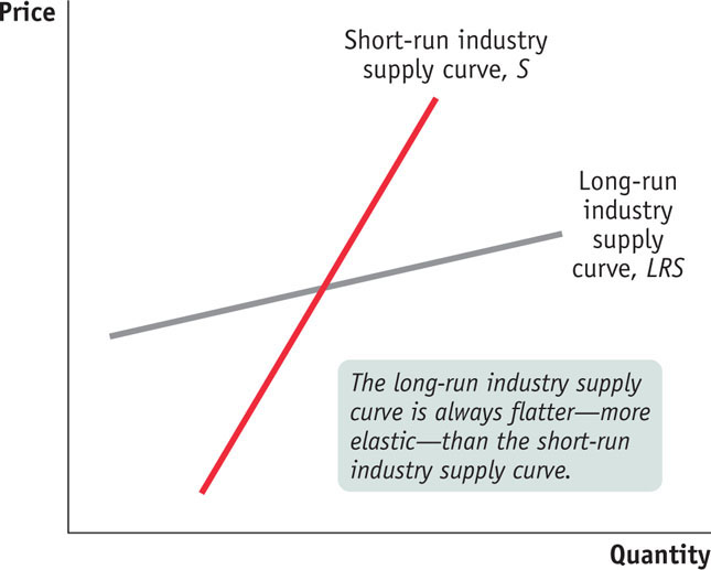
Regardless of whether the long-run industry supply curve is horizontal, upward sloping, or downward sloping, the long-run price elasticity of supply is higher than the short-run price elasticity whenever there is free entry and exit. As shown in Figure 27-5, the long-run industry supply curve is always flatter than the short-run industry supply curve. The reason is entry and exit: a high price caused by an increase in demand attracts entry by new firms, resulting in a rise in industry output and an eventual fall in price; a low price caused by a decrease in demand induces existing firms to exit, leading to a fall in industry output and an eventual increase in price.

The long-run industry supply curve may slope upward, but it is always flatter—more elastic—than the short-run industry supply curve. This is because of entry and exit: a higher price attracts new entrants in the long run, resulting in a rise in industry output and a fall in price; a lower price induces existing producers to exit in the long run, generating a fall in industry output and a rise in price.

Firms producing electric cars enjoy decreasing costs across the industry.

Simon Turner/Alamy

The distinction between the short-run industry supply curve and the long-run industry supply curve is very important in practice. We often see a sequence of events like that shown in Figure 27-4: an increase in demand initially leads to a large price increase, but prices return to their initial level once new firms have entered the industry. Or we see the sequence in reverse: a fall in demand reduces prices in the short run, but they return to their initial level as producers exit the industry.

The Cost of Production and Efficiency in Long-Run Equilibrium

Our analysis leads us to three conclusions about the cost of production and efficiency in the long-run equilibrium of a perfectly competitive industry. These results will be important in our upcoming discussion of how monopoly gives rise to inefficiency.

First, in a perfectly competitive industry in equilibrium, the value of marginal cost is the same for all firms. That’s because all firms produce the quantity of output at which marginal cost equals the market price, and as price-takers they all face the same market price.

Second, in a perfectly competitive industry with free entry and exit, each firm will have zero economic profit in the long-run equilibrium. Each firm produces the quantity of output that minimizes its average total cost—corresponding to point Z in panel (c) of Figure 27-4. So the total cost of producing the industry’s output is minimized in a perfectly competitive industry.

The third and final conclusion is that the long-run market equilibrium of a perfectly competitive industry is efficient: no mutually beneficial transactions go unexploited. To understand this, recall a fundamental requirement for efficiency: all consumers who are willing to pay an amount greater than or equal to the sellers’ cost actually get the good. We also learned that when a market is efficient (except under certain, well-defined conditions), the market price matches all consumers willing to pay at least the market price with all sellers who have a cost of production that is less than or equal to the market price.

So in the long-run equilibrium of a perfectly competitive industry, production is efficient: costs are minimized and no resources are wasted. In addition, the allocation of goods to consumers is efficient: every consumer willing to pay the cost of producing the good gets it. Indeed, no mutually beneficial transaction is left unexploited. Moreover, this condition tends to persist over time as the environment changes: the force of competition makes producers responsive to changes in consumers’ desires and to changes in technology.

Module 27 Review

Check Your Understanding

Draw correctly labeled side-by-side graphs to show the long-run adjustment that would take place if perfectly competitive firms were earning a profit.