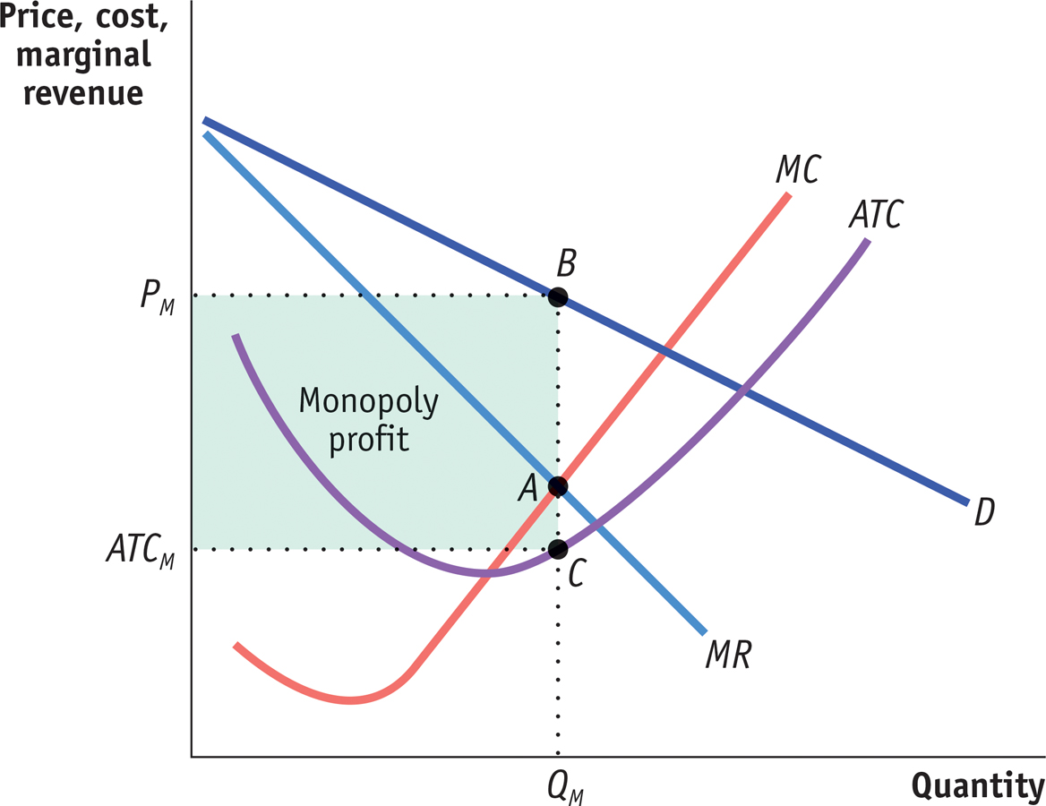
Figure 13-6 involved specific numbers and assumed that marginal cost was constant, that there was no fixed cost, and, therefore, that the average total cost curve was a horizontal line. Figure 13-7 shows a more general picture of monopoly in action: D is the market demand curve; MR, the marginal revenue curve; MC, the marginal cost curve; and ATC, the average total cost curve. Here we return to the usual assumption that the marginal cost curve has a “swoosh” shape and the average total cost curve is ∪-shaped.

Applying the optimal output rule, we see that the profit-maximizing level of output is the output at which marginal revenue equals marginal cost, indicated by point A. The profit-maximizing quantity of output is Q_M, and the price charged by the monopolist is P_M. At the profit-maximizing level of output, the monopolist’s average total cost is ATC_M, shown by point C.

Recalling how we calculated profit in Equation 12-5, profit is equal to the difference between total revenue and total cost. So we have:

Profit is equal to the area of the shaded rectangle in Figure 13-7, with a height of P_M − ATC_M and a width of Q_M.

13-7

The Monopolist’s Profit

In Chapter 12 we learned that a perfectly competitive industry can have profits in the short run but not in the long run. In the short run, price can exceed average total cost, allowing a perfectly competitive firm to make a profit. But we also know that this cannot persist.

In the long run, any profit in a perfectly competitive industry will be competed away as new firms enter the market. In contrast, barriers to entry allow a monopolist to make profits in both the short run and the long run.

One major obstacle to lowering electricity prices through deregulation is the lack of choice in power generators, the bulk of which still entail large up-front fixed costs. As a result, in many markets there is only one power generator. Although consumers appear to have a choice in their electricity distributor, the choice is illusory, as everyone must get their electricity from the same source in the end.

In fact, deregulation can make consumers worse off when there is only one power generator. That’s because deregulation allows the power generator to engage in market manipulation—intentionally reducing the amount of power supplied to distributors in order to drive up prices. The most shocking case occurred during the California energy crisis of 2000–2001 that brought blackouts and billions of dollars in electricity surcharges to homes and businesses. On audiotapes later acquired by regulators, workers could be heard discussing plans to shut down power plants during times of peak energy demand, joking about how they were “stealing” more than $1 million a day from California.

Another problem is that without prices set by regulators, producers aren’t guaranteed a profitable rate of return on new power plants. As a result, in states with deregulation, capacity has failed to keep up with growing demand. For example, Texas, a deregulated state, has experienced massive blackouts due to insufficient capacity, and in New Jersey and Maryland, regulators have intervened to compel producers to build more power plants.

Lastly, consumers in deregulated states have been subject to big spikes in their electricity bills, often paying much more than consumers in regulated states. So, angry customers and exasperated regulators have prompted many states to shift into reverse, with Illinois, Montana, and Virginia moving to regulate their industries. California and Montana have gone so far as to mandate that their electricity distributors reacquire power plants that were sold off during deregulation. In addition, regulators have been on the prowl, fining utilities in Texas, New York, and Illinois for market manipulation.