Suppose that Clive’s wage rate doubles, from $10 to $20 per hour. How will he change his time allocation?

You could argue that Clive will work longer hours, because his incentive to work has increased: by giving up an hour of leisure, he can now gain twice as much money as before. But you could equally well argue that he will work less, because he doesn’t need to work as many hours to generate the income to pay for the goods he wants.

As these opposing arguments suggest, the quantity of labor Clive supplies can either rise or fall when his wage rate rises. To understand why, let’s recall the distinction between substitution effects and income effects that we learned in Chapter 10 and its appendix. We saw there that a price change affects consumer choice in two ways: by changing the opportunity cost of a good in terms of other goods (the substitution effect) and by making the consumer richer or poorer (the income effect).

Now think about how a rise in Clive’s wage rate affects his demand for leisure. The opportunity cost of leisure—the amount of money he gives up by taking an hour off instead of working—rises. That substitution effect gives him an incentive, other things equal, to consume less leisure and work longer hours. Conversely, a higher wage rate makes Clive richer—and this income effect leads him, other things equal, to want to consume more leisure and work fewer hours, because leisure is a normal good.

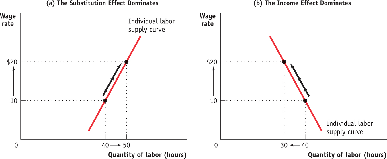
So in the case of labor supply, the substitution effect and the income effect work in opposite directions. If the substitution effect is so powerful that it dominates the income effect, an increase in Clive’s wage rate leads him to supply more hours of labor. If the income effect is so powerful that it dominates the substitution effect, an increase in the wage rate leads him to supply fewer hours of labor.

We see, then, that the individual labor supply curve—the relationship between the wage rate and the number of hours of labor supplied by an individual worker—does not necessarily slope upward. If the income effect dominates, a higher wage rate will reduce the quantity of labor supplied.

Figure 19-11 illustrates the two possibilities for labor supply. If the substitution effect dominates the income effect, the individual labor supply curve slopes upward; panel (a) shows an increase in the wage rate from $10 to $20 per hour leading to a rise in the number of hours worked from 40 to 50. However, if the income effect dominates, the quantity of labor supplied goes down when the wage rate increases. Panel (b) shows the same rise in the wage rate leading to a fall in the number of hours worked from 40 to 30. (Economists refer to an individual labor supply curve that contains both upward-sloping and downward-sloping segments as a “backward-bending labor supply curve”—a concept that we analyze in detail in this chapter’s appendix.)

Is a negative response of the quantity of labor supplied to the wage rate a real possibility? Yes: many labor economists believe that income effects on the supply of labor may be somewhat stronger than substitution effects. The most compelling piece of evidence for this belief comes from Americans’ increasing consumption of leisure over the past century. At the end of the nineteenth century, wages adjusted for inflation were only about one-eighth what they are today; the typical workweek was 70 hours, and very few workers retired at age 65. Today the typical workweek is less than 40 hours, and most people retire at age 65 or earlier. So it seems that Americans have chosen to take advantage of higher wages in part by consuming more leisure.