An Alternative Way to Calculate Elasticities: The Midpoint Method
Price elasticity of demand compares the percent change in quantity demanded with the percent change in price. When we look at some other elasticities, which we will do shortly, we’ll learn why it is important to focus on percent changes. But at this point we need to discuss a technical issue that arises when you calculate percent changes in variables.
The best way to understand the issue is with a real example. Suppose you were trying to estimate the price elasticity of demand for gasoline by comparing gasoline prices and consumption in different countries. Because of high taxes, gasoline usually costs about three times as much per gallon in Europe as it does in the United States. So what is the percent difference between American and European gas prices?
Well, it depends on which way you measure it. Because the price of gasoline in Europe is approximately three times higher than in the United States, it is 200 percent higher. Because the price of gasoline in the United States is one-
This is a nuisance: we’d like to have a percent measure of the difference in prices that doesn’t depend on which way you measure it. To avoid computing different elasticities for rising and falling prices we use the midpoint method.
The midpoint method is a technique for calculating the percent change. In this approach, we calculate changes in a variable compared with the average, or midpoint, of the starting and final values.
The midpoint method replaces the usual definition of the percent change in a variable, X, with a slightly different definition:
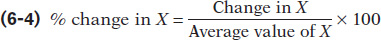
where the average value of X is defined as

When calculating the price elasticity of demand using the midpoint method, both the percent change in the price and the percent change in the quantity demanded are found using this method. To see how this method works, suppose you have the following data for some good:
|
Price |
Quantity demanded |
|
|
Situation A |
$0.90 |
1,100 |
|
Situation B |
$1.10 |
900 |
To calculate the percent change in quantity going from situation A to situation B, we compare the change in the quantity demanded—

In the same way, we calculate

So in this case we would calculate the price elasticity of demand to be

again dropping the minus sign.
The important point is that we would get the same result, a price elasticity of demand of 1, whether we go up the demand curve from situation A to situation B or down from situation B to situation A.
To arrive at a more general formula for price elasticity of demand, suppose that we have data for two points on a demand curve. At point 1 the quantity demanded and price are (Q1, P1); at point 2 they are (Q2, P2). Then the formula for calculating the price elasticity of demand is:

As before, when finding a price elasticity of demand calculated by the midpoint method, we drop the minus sign and use the absolute value.
ECONOMICS in Action: Estimating Elasticities
Estimating Elasticities
6-1
Some Estimated Price Elasticities of Demand
|
Good |
Price elasticity of demand |
|---|---|
|
Inelastic demand |
|
|
Gasoline (short- |
0.09 |
|
Gasonline (long- |
0.24 |
|
Airline travel (business) |
0.80 |
|
Soda |
0.80 |
|
College (in- |
0.87 |
|
Elastic demand |
|
|
Housing |
1.2 |
|
College (out- |
1.2 |
|
Airline travel (leisure) |
1.5 |
|
Coke/Pepsi |
3.3 |
TABLE 6-
You might think it’s easy to estimate price elasticities of demand from real-
To estimate price elasticities of demand, economists must use careful statistical analysis to separate the influence of the change in price, holding other things equal.
Economists have estimated price elasticities of demand for a number of goods and services. Table 6-1 summarizes some of these and shows a wide range of price elasticities. There are some goods, like gasoline for which demand hardly responds at all to changes in the price. There are other goods, such as airline travel for leisure, or Coke and Pepsi, for which the quantity demanded is very sensitive to the price.
Notice that Table 6-1 is divided into two parts: inelastic and elastic demand. We’ll explain the significance of that division in the next section.
Quick Review
The price elasticity of demand is equal to the percent change in the quantity demanded divided by the percent change in the price as you move along the demand curve, and dropping any minus sign.
In practice, percent changes are best measured using the midpoint method, in which the percent changes are calculated using the average of starting and final values.
6-1
Question 6.1
The price of strawberries falls from $1.50 to $1.00 per carton and the quantity demanded goes from 100,000 to 200,000 cartons. Use the midpoint method to find the price elasticity of demand.
Question 6.2
At the present level of consumption, 4,000 movie tickets, and at the current price, $5 per ticket, the price elasticity of demand for movie tickets is 1. Using the midpoint method, calculate the percentage by which the owners of movie theaters must reduce price in order to sell 5,000 tickets.
Question 6.3
The price elasticity of demand for ice-
cream sandwiches is 1.2 at the current price of $0.50 per sandwich and the current consumption level of 100,000 sandwiches. Calculate the change in the quantity demanded when price rises by $0.05. Use Equations 6- 1 and 6- 2 to calculate percent changes and Equation 6- 3 to relate price elasticity of demand to the percent changes.
Solutions appear at back of book.