Life tables keep track of demographic events
Up to this point we have assumed that individuals within a population do not vary in their birth and death rates. This is a big assumption given that we know real populations are made up of individuals of different ages, sizes, and sexes, which vary in their capacity to reproduce or survive. For example, a newborn whale or human cannot reproduce immediately, but must mature to reproductive age. Likewise, the likelihood of death will vary depending on the age of the individual. Ecologists use a form of accounting, known as a life table, to keep track of how demography will affect the growth rate of the population. Life tables summarize how survival and reproductive rates vary with the age, size, or sex of the individuals within a population. These summaries can then be used to predict future population trends and develop strategies for managing populations of commercial or ecological value. They are also used by life insurance companies to determine how much to charge people of different ages for insurance policies.
Let’s consider an example of a life table from the literature. Table 54.1 shows a cohort life table using data from the acorn barnacle Balanus glandula on the shorelines of Scotland. A cohort life table uses a cohort—
R0 = sum (lx mx) (54.8)
If R0 is greater than 1.0, there is a net increase in offspring produced each generation, and assuming the birth and death rates do not change over time, the population should increase exponentially. If R0 is less than 1.0, and individuals are not replaced as they die, the population declines eventually to extinction. If R0 is 1.0, then the births and deaths balance out and the population will not change in size.
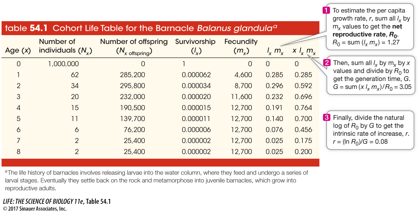
We can use R0 to estimate the per capita growth rate, r, of a cohort by scaling R0 to account for the generation time of the cohort. The generation time, G, is the average age of the parents of all the offspring produced within the cohort (see Table 54.1 for equation). To estimate r, we simply divide the natural log (ln) of R0 by G and get
r = (ln R0)/G (54.9)
Cohort life tables follow individuals from birth to death as a function of calendar year or life stage (e.g., eggs, larvae, pupae, and adults in insects). This is relatively easy to do if the organisms are easily followed—
The construction of life tables has allowed ecologists to observe common life history patterns, reflecting common solutions to ecological challenges, across a tremendous diversity of organisms. For example, the number of individuals surviving through each life stage (survivorship, lx) can be taken from a life table and plotted graphically to construct a survivorship curve. Typically, a survivorship curve is constructed for a hypothetical cohort, usually of 1,000 individuals, by plotting the numbers of individuals expected to survive to reach each age category on a logarithmic scale.
Survivorship curves tend to take one of three general shapes:
Species with type I survivorship curves experience high overall survivorship through adulthood but steep declines late in life (the curve is concave) (Figure 54.9A). Species with this type of survivorship curve (humans, elephants, whales, and many other large mammals) typically have low reproduction rates but provide parental care to their offspring, which reduces the risk of death in early stages of development.
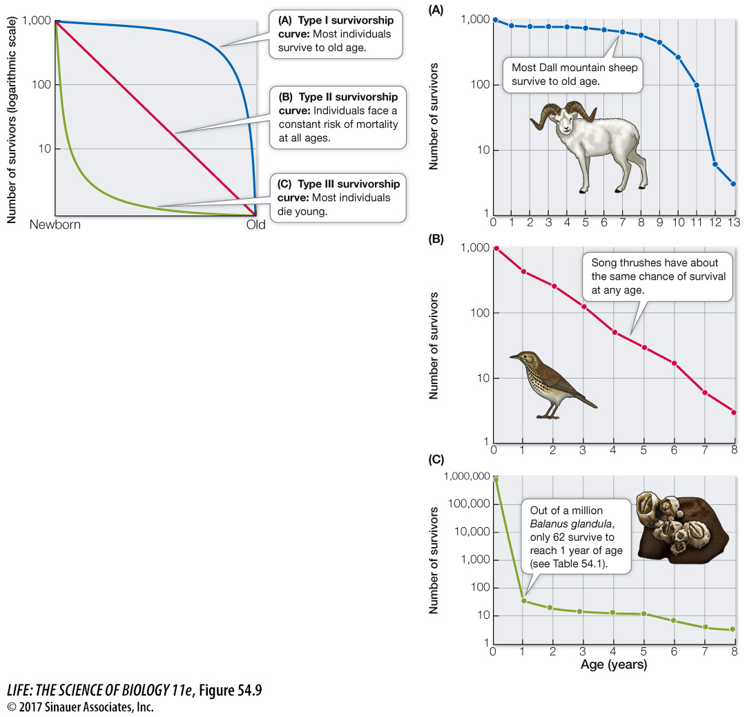 Figure 54.9 Survivorship Curves Ecologists recognize three general types of survivorship curves. Notice that the number of survivors has been plotted on a logarithmic scale. Three species provide real-
world examples of the three types of life histories. Q: What type of survivorship curve do humans have?
Humans have a type I survivorship because they have high overall survivorship through adulthood but a steep decline later in life. Species with this type of survivorship curve typically have low reproduction rates but provide parental care to their offspring, which reduces the risk of death in early stages of development.
Activity 54.4 Age Structure and Survivorship Simulation
Species with type II survivorship curves face a constant risk of mortality at all ages (the curve is linear) (Figure 54.9B). Many birds, fish, and plants display this pattern.
Species with type III survivorship curves experience low survivorship early in life and higher survivorship once they reach maturity (the curve is convex) (Figure 54.9C). Species with this type of survivorship curve (most insects; marine invertebrates, including the barnacle in Table 54.1; and annual plants) tend to produce many offspring but provide little or no parental care.
Species survivorship curves help us classify how mortality plays out in populations over time, but many species have patterns of survivorship somewhere in between these extremes. For example, some organisms show a “stair-