Step 5: Make Inferences from the Data
Data analysis often culminates with statistical inference—
STATISTICAL HYPOTHESES Once we have collected our data, we want to evaluate whether or not they fit the predictions of our hypothesis. For example, we want to know whether or not cancer incidence is greater in our sample of smokers than in our sample of nonsmokers, whether or not clutch size increases with spider body weight in our sample of spiders, or whether or not growth of a sample of fertilized plants is greater than that of a sample of unfertilized plants.
Before making statistical inferences from data, we must formalize our “whether or not” question into a pair of opposing hypotheses. We start with the “or not” hypothesis, which we call the null hypothesis (denoted H0) because it often is the hypothesis that there is no difference between sample means, no correlation between variables in the sample, or no difference between our sample and an expected frequency distribution. The alternative hypothesis (denoted HA) is that there is a difference in means, that there is a correlation between variables, or that the sample distribution does differ from the expected one.
Suppose, for example, we would like to know whether or not a new vaccine is more effective than an existing vaccine at immunizing children against influenza. We have measured flu incidence in a group of children who received the new vaccine and want to compare it with flu incidence in a group of children who received the old vaccine. Our statistical hypotheses would be as follows:
H0: Flu incidence was the same in both groups of children.
HA: Flu incidence was different between the two groups of children.
In the next few sections we will discuss how we decide when to reject the null hypothesis in favor of the alternative hypothesis.
JUMPING TO THE WRONG CONCLUSIONS There are two ways that a statistical test can go wrong (Figure B10). We can reject the null hypothesis when it is actually true (Type I error), or we can accept the null hypothesis when it is actually false (Type II error). These kinds of errors are analogous to false positives and false negatives in medical testing, respectively. If we mistakenly reject the null hypothesis when it is actually true, then we falsely endorse the incorrect hypothesis. If we are unable to reject the null hypothesis when it is actually false, then we fail to realize a yet undiscovered truth.
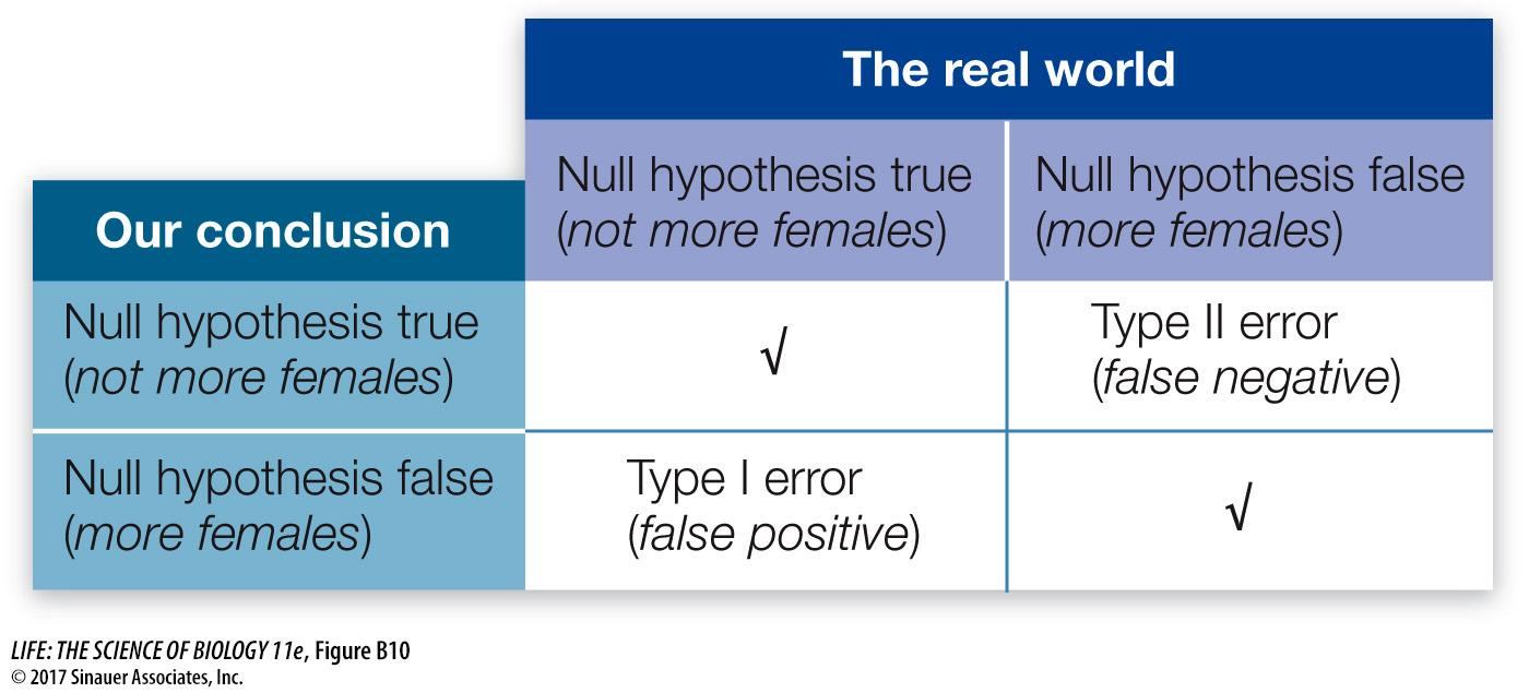
Suppose we would like to know whether there are more females than males in a population of 10,000 individuals. To determine the makeup of the population, we choose 20 individuals randomly and record their sex. Our null hypothesis is that there are not more females than males; and our alternative hypothesis is that there are. The following scenarios illustrate the possible mistakes we might make:
Scenario 1: The population actually has 40% females and 60% males. Although our random sample of 20 people is likely to be dominated by males, it is certainly possible that, by chance, we will end up choosing more females than males. If this occurs, and we mistakenly reject the null hypothesis (that there are not more females than males), then we make a Type I error.
Scenario 2: The population actually has 60% females and 40% males. If, by chance, we end up with a majority of males in our sample and thus fail to reject the null hypothesis, then we make a Type II error.
Fortunately, statistics has been developed precisely to avoid these kinds of errors and inform us about the reliability of our conclusions. The methods are based on calculating the probabilities of different possible outcomes. Although you may have heard or even used the word “probability” on multiple occasions, it is important that you understand its mathematical meaning. A probability is a numerical quantity that expresses the likelihood of some event. It ranges between zero and 1; zero means there is no chance the event will occur, and 1 means the event is guaranteed to occur. This only makes sense if there is an element of chance, that is, if it is possible the event will occur and possible that it will not occur. For example, when we flip a fair coin, it will land on heads with probability 0.5 and land on tails with probability 0.5. When we select individuals randomly from a population with 60% females and 40% males, we will encounter a female with probability 0.6 and a male with probability 0.4.
Probability plays a very important role in statistics. To draw conclusions about the real world (the population) from our sample, we first calculate the probability of obtaining our sample if the null hypothesis is true. Specifically, statistical inference is based on answering the following question:
Suppose the null hypothesis is true. What is the probability that a random sample would, by chance, differ from the null hypothesis as much as our sample differs from the null hypothesis?
If our sample is highly improbable under the null hypothesis, then we rule it out in favor of our alternative hypothesis. If, instead, our sample has a reasonable probability of occurring under the null hypothesis, then we conclude that our data are consistent with the null hypothesis and we do not reject it.
Returning to the sex ratio example, let’s consider two new scenarios:
Scenario 3: Suppose we want to infer whether or not females constitute the majority of the population (our alternative hypothesis) based on a random sample containing 12 females and 8 males. We would calculate the probability that a random sample of 20 people includes at least 12 females assuming that the population, in fact, has a 50:50 sex ratio (our null hypothesis). This probability is 0.13, which is too high to rule out the null hypothesis.
Scenario 4: Suppose now that our sample contains 17 females and 3 males. If our population is truly evenly divided, then this sample is much less likely than the sample in scenario 3. The probability of such an extreme sample is 0.0002, and would lead us to rule out the null hypothesis and conclude that there are more females than males.
This agrees with our intuition. When choosing 20 people randomly from an evenly divided population, we would be surprised if almost all of them were female, but would not be surprised at all if we ended up with a few more females than males (or a few more males than females). Exactly how many females do we need in our sample before we can confidently infer that they make up the majority of the population? And how confident are we when we reach that conclusion? Statistics allows us to answer these questions precisely.
STATISTICAL SIGNIFICANCE: AVOIDING FALSE POSITIVES Whenever we test hypotheses, we calculate the probability just discussed, and refer to this value as the P-value of our test. Specifically, the P-value is the probability of getting data as extreme as our data (just by chance) if the null hypothesis is in fact true. In other words, it is the likelihood that chance alone would produce data that differ from the null hypothesis as much as our data differ from the null hypothesis. How we measure the difference between our data and the null hypothesis depends on the kind of data in our sample (categorical or quantitative) and the nature of the null hypothesis (assertions about proportions, single variables, multiple variables, differences between variables, correlations between variables, etc.).
For many statistical tests, P-values can be calculated mathematically. One option is to quantify the extent to which the data depart from the null hypothesis and then use look-
After we calculate a P-value from our data, we have to decide whether it is small enough to conclude that our data are inconsistent with the null hypothesis. This is decided by comparing the P-value to a threshold called the significance level, which is often chosen even before making any calculations. We reject the null hypothesis only when the P-value is less than or equal to the significance level, denoted α. This ensures that, if the null hypothesis is true, we have at most a probability α of accidentally rejecting it. Therefore the lower the value of α, the less likely we are to make a Type I error (see the lower left cell of Figure B10). The most commonly used significance level is α = 0.05, which limits the probability of a Type I error to 5%.
If our statistical test yields a P-value that is less than our significance level α, then we conclude that the effect described by our alternative hypothesis is statistically significant at the level α and we reject the null hypothesis. If our P-value is greater than α, then we conclude that we are unable to reject the null hypothesis. In this case, we do not actually reject the alternative hypothesis, rather we conclude that we do not yet have enough evidence to support it.
POWER: AVOIDING FALSE NEGATIVES The power of a statistical test is the probability that we will correctly reject the null hypothesis when it is false (see the lower right cell of Figure B10). Therefore the higher the power of the test, the less likely we are to make a Type II error (see the upper right cell of Figure B10). The power of a test can be calculated, and such calculations can be used to improve your methodology. Generally, there are several steps that can be taken to increase power and thereby avoid false negatives:
Decrease the significance level, α. The higher the value of α, the harder it is to reject the null hypothesis, even if it is actually false.
Increase the sample size. The more data one has, the more likely one is to find evidence against the null hypothesis, if it is actually false.
Decrease variability in the sample. The more variation there is in the sample, the harder it is to discern a clear effect (the alternative hypothesis) when it actually exists.
It is always a good idea to design your experiment to reduce any variability that may obscure the pattern you seek to detect. For example, it is possible that the chance of a child contracting influenza varies depending on whether he or she lives in a crowded (e.g., urban) environment or one that is less so (e.g., rural). To reduce variability, a scientist might choose to test a new influenza vaccine only on children from one environment or the other. After you have minimized such extraneous variation, you can use power calculations to choose the right combination of α and sample size to reduce the risks of Type I and Type II errors to desirable levels.
There is a trade-
STATISTICAL INFERENCE WITH QUANTITATIVE DATA Statistics that describe patterns in our samples are used to estimate properties of the larger population. Earlier we calculated the mean weight of a sample of Abramis brama in Lake Laengelmavesi, which provided us with an estimate of the mean weight of all the Abramis brama in the lake. But how close is our estimate to the true value in the larger population? Our estimate from the sample is unlikely to exactly equal the true population value. For example, our sample of Abramis brama may, by chance, have included an excess of large individuals. In this case, our sample would overestimate the true mean weight of fish in the population.
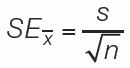
The standard error of a sample statistic (such as the mean) is a measure of how close it is likely to be to the true population value. The standard error of the mean, for example, provides an estimate of how far we might expect a sample mean to deviate from the true population mean. It is a function of how much individual observations vary within samples (the standard deviation) and the size of the sample (n). Standard errors increase with the degree of variation within samples, and they decrease with the number of observations in a sample (because large samples provide better estimates about the underlying population than do small samples). For our sample of 34 Abramis brama, we would calculate the standard error of the mean using equation 5 in Figure B6:
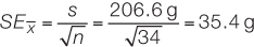
The standard error of a statistic is related to the confidence interval—a range around the sample statistic that has a specified probability of including the true population value. The formula we use to calculate confidence intervals depends on the characteristics of the data, and the particular statistic. For many types of continuous data, the bounds of the 95% confidence interval of the mean can be calculated by taking the mean and adding and subtracting 1.96 times the standard error of the mean. Consider our sample of 34 Abramis brama, for example. We would say that the mean of 626 g has a 95% confidence interval from 556.6 g to 695.4 g (626 ± 69.4 g). If all our assumptions about our data have been met, we would expect the true population mean to fall in this confidence interval 95% of the time.
Researchers typically use graphs or tables to report sample statistics (such as the mean) as well as some measure of confidence in them (such as their standard error or a confidence interval). This book is full of examples. If you understand the concepts of sample statistics, standard errors, and confidence intervals, you can see for yourself the major patterns in the data, without waiting for the authors to tell you what they are. For example, if samples from two groups have 95% confidence intervals of the mean that do not overlap, then you can conclude that it is unlikely that the groups have the same true mean.
Activity B1 Standard Deviations, Standard Errors, and Confidence Intervals Simulation
Biologists conduct statistical tests to obtain more precise estimates of the probability of observing a given difference between samples if the null hypothesis that there is no difference in the populations is true. The appropriate test depends on the nature of the data and the experimental design. For example, we might want to calculate the probability that the mean weights of two different fish species in Lake Laengelmavesi, Abramis brama and Leusiscus idus, are the same. A simple method for comparing the means of two groups is the t-test, described in Figure B11. We looked earlier at data for Abramis brama; the researchers who collected these data also collected weights for six individuals of Leusiscus idus: 270, 270, 306, 540, 800, and 1,000 g. We begin by stating our hypotheses and choosing a significance level:
H0: Abramis brama and Leusiscus idus have the same mean weight.
HA: Abramis brama and Leusiscus idus have different mean weights.
α = 0.05
The test statistic is calculated using the means, standard deviations, and sizes of the two samples:
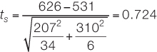
We can use statistical software or one of the free statistical sites on the internet to find that the P-value for this result is P = 0.497. Since P is considerably greater than α, we fail to reject the null hypothesis and conclude that our study does not provide evidence that the two species have different mean weights.
research tools
Figure B11 The t-test What is the t-test? It is a standard method for assessing whether the means of two groups are statistically different from each other.
Step 1:
State the null and alternative hypotheses:
H0: The two populations have the same mean.
HA: The two populations have different means.
Step 2:
Choose a significance level, α, to limit the risk of a Type I error.
Step 3:
Calculate the test statistic:
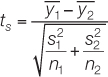
Notation: y1 and y2 are the sample means; s1 and s2 are the sample standard deviations; and n1 and n2 are the sample sizes.
Step 4:
Use the test statistic to assess whether the data are consistent with the null hypothesis:
Calculate the P-value (P) using statistical software or by hand using statistical tables.
Step 5:
Draw conclusions from the test:
If P ≤ α, then reject H0, and conclude that the population distribution is significantly different.
If P > α, then we do not have sufficient evidence to conclude that the means differ.
You may want to consult an introductory statistics textbook to learn more about confidence intervals, t-tests, and other basic statistical tests for quantitative data.
STATISTICAL INFERENCE WITH CATEGORICAL DATA With categorical data, we often wish to ask whether the frequencies of observations in different categories are consistent with a hypothesized frequency distribution. We can use a chi-
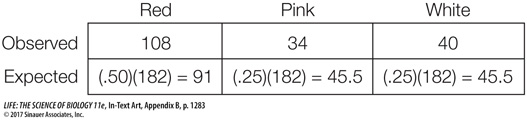
Figure B12 outlines the steps of a chi-
H0: The progeny of this type of cross have the following probabilities of each flower color:
Pr{Red} = 0.50, Pr{Pink} = 0.25, Pr{White} = 0.25
HA: At least one of the probabilities of H0 is incorrect.
α = 0.05
We next use the probabilities in H0 and the sample size to calculate the expected frequencies:
Based on these quantities, we calculate the chi-
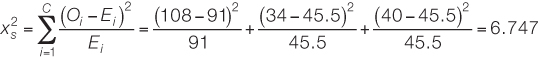
We find the P-value for this result to be P = 0.034 using statistical software. Since P is less than α, we reject the null hypothesis and conclude that the botanist is likely correct: the plant color patterns are not explained by the simple Mendelian genetic model under consideration.
research tools
Figure B12 The Chi-
Step 1:
State the null and alternative hypotheses:
H0: The population has the specified distribution.
HA: The population does not have the specified distribution.
Step 2:
Choose a significance level, α, to limit the risk of a Type I error.
Step 3:
Determine the observed frequency and expected frequency for each category:
The observed frequency of a category is simply the number of observations in the sample of that type.
The expected frequency of a category is the probability of the category specified in H0 multiplied by the overall sample size.
Step 4:
Calculate the test statistic:
Notation: C is the total number of categories, Oi is the observed frequency of category i, and E1 is the expected frequency of category i.
Step 5:
Use the test statistic to assess whether the data are consistent with the null hypothesis:
Calculate the P-value (P) using statistical software or by hand using statistical tables.
Step 6:
Draw conclusions from the test:
If P ≤ α, then reject H0, and conclude that the population distribution is significantly different than the distribution specified by H0.
If P > α, then we do not have sufficient evidence to conclude that population has a different distribution.
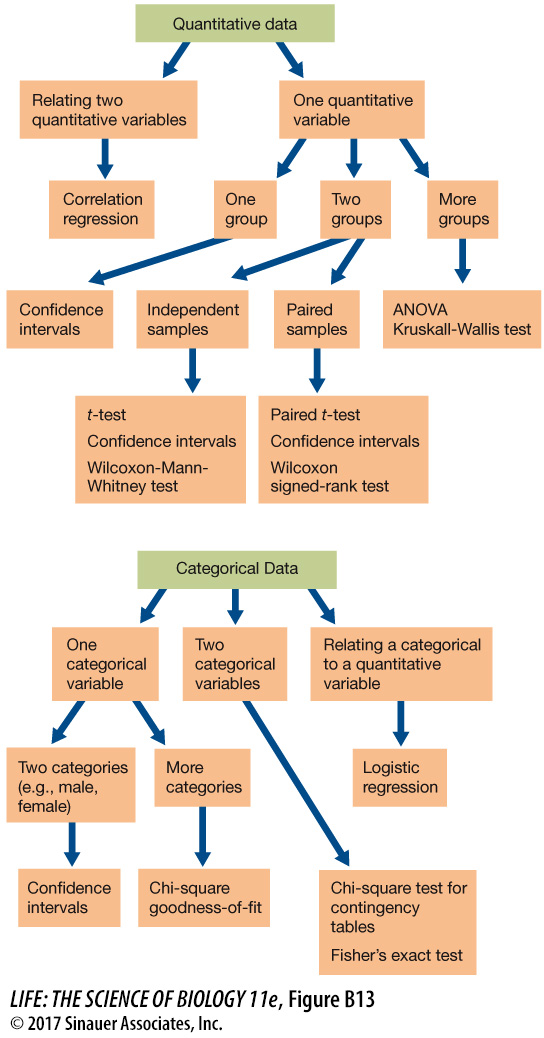
This introduction is meant to provide only a brief introduction to the concepts of statistical analysis, with a few example tests. Figure B13 summarizes some of the commonly used statistical tests that you may encounter in biological studies.