Chapter 54

1. 

   Yes, the five populations of humpback whales make up one metapopulation on their summer feeding grounds. All populations except the yellow and blue populations overlap in their summer feeding areas and thus have the potential to exchange individuals. The yellow and blue populations overlap with the other three populations, however, so they are still part of the metapopulation.

2. Intraspecific competition for food resources is likely responsible for fluctuations in the aphid population size over time. Aphid populations undergo boom-and-bust cycles triggered by their population densities. Predation keeps these fluctuations in check by controlling the density of aphids before they reach boom-and-bust conditions.

3. Approaches used to estimate population sizes include full censuses, surveys using quadrats or transects, mark–recapture methods, and DNA analyses.

4. The most appropriate method would probably be mark–recapture. Quadrats and transects are appropriate only for plants and sessile animals. In a large area, or in water, it is impractical or impossible to do a full census. For animals that can move, the best approach is to collect a sample of animals, mark them, and then recapture them and count the marked organisms. This allows the researcher to calculate a reasonable estimate of the population.

1. 1. N_t = N₀ + (B – D) + (I – E)

      N_t = population size at time t; N₀ = population size at time 0; B = number of individuals born between time 0 and time t: D = number of individuals that died between time 0 and time t; I = number of individuals that immigrated between time 0 and time t; E = number of individuals that emigrated between time 0 and time t.

2. 1.  

      Year	Age (x)	Number of female birds (Nx)	Number of female offspring (Nx offspring)	Survivorship (lx)	Fecundity (mx)	Net reproductive rate (lx mx)	Generation time (x lx mx)
      2012	0	100	0	0	0	0	0
      2013	1	50	75	0.50	1.50	0.75	0.75
      2014	2	40	80	0.40	2.00	0.80	1.60
      2015	3	30	60	0.30	2.00	0.60	1.80
      						R0 = 2.15	4.15

   2. R₀ = 2.15; G = 4.15/2.15 = 1.93; r = ln (2.15)/1.93 = 0.40.

   3. N_t = (120) e ^{0.40 × 20} = (120)(2,982) = 357,720.

   4. N_t = 300/(1 + [(300 – 120)/120] e^{–0.40 × 20}) = 300/1.0005 = 300.

3. 

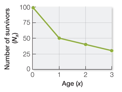
   This cohort has a type II survivorship curve, which is typical for birds, fish, and plants.

4. Density-dependent factors controlling this cohort could include limiting resources that decrease population growth under high densities as a result of intraspecific competition; and predators or pathogens that can have a differential effect on the mortality of individuals in high population densities. Density-independent factors controlling this cohort could include extreme cold or an exceptionally strong hurricane that kills a large number of individuals in the population.

1. 1. Life expectancy has increased steadily over the past 175 years, suggesting that advances in food and health security (i.e., environmental factors) have allowed humans to live longer. Changes in genetically determined life span would occur over evolutionary time.

   2. The differences in life span for citizens of Japan versus Angola are also mostly the result of environmental factors. Citizens of Japan generally have a better quality of life than those of Angola, due to Angola’s high rates of HIV infection and civil unrest.

2. There are life history trade-offs because constraints on optimality include genetic variation for evolution to act on as well as the mediating effects of the physical and biological environments. Examples of trade-offs are allocation of resources, high growth versus high reproduction, and high reproduction versus survival.

3. Lobelia telekii reproduces just once, produces many seeds, and has a short life span, which falls on the side of an r-strategist. L. keniensis reproduces multiple times, produces fewer but larger seeds, and lives longer, suggesting a K-strategist life history. In terms of the guppy example, those living in high-predation streams have an r-strategist life history whereas those living in low-predation streams have a more K-strategist life history.

1. Species that have a K-strategist life history live longer, reproduce at a larger size, and produce fewer offspring over a longer period of time compared to r-strategists. As a result, recovery may require managing the number or size of the individuals within the population so that they live long enough, and/or reach a large enough size, to successfully reproduce at a rate that increases their population size over time.

2. 1. Some factors that affect the metapopulation size of the Edith’s checkerspot butterfly in the San Francisco Bay area include the number and size of serpentine rock outcrops with the host plants of the butterfly, the effects of climate on the populations, the dispersal rates between the populations, and the number of source and sink populations.

   2. With the extinction of the Morgan Hill population, the metapopulation faces likely extinction. Large populations, such as Morgan Hill, serve as sources that recolonize smaller populations after temporary local extinctions. Without such source populations, continuation of the metapopulation over the long term is much less likely.

1. The equation in Figure 54.5A states that N = (n₁ × n₂)/M. In words, the estimated total number of ticks (population size N) equals the total number of individuals captured, marked, and released in the first sample (n₁ = 180) times the total number of individuals captured in the second sample (n₂ = 33) divided by the number of marked individuals recaptured in the second sample (M = 8). Thus N (estimated population of the sampled lawn) = (180 × 33)/8 = 5,940/8 = 742.5 adult ticks.

2. Calculate this by dividing 742.5 (the estimated number of ticks in the lawn population, per Question 1) by 700 (number of m²) = approximately 1.06 ticks per square meter.

3. This study was conducted in order to evaluate the risk that residents of this suburban neighborhood have of encountering the tick vectors of Lyme disease in their own yards; a high risk of encounter means that there is also likely to be a high risk of contracting the disease. A density of slightly more than one tick per square meter of lawn suggests that residents of this community are indeed likely to encounter ticks and, accordingly, have a high probability of contracting Lyme disease if they spend time outdoors on their lawns.

1. N_t = (7.4 billion) e^{0.0118 × 85} = (7.4)(2.73) = 20.2 billion.

2. N_t = (10 billion)e^{0.005 × 20} = (10)(1.01) = 10.1 billion.

3. 2015 data: N_t = 12 /[1 + ([12 – 7.4]/12)e^{–0.0118 × 85}] = 12/1.14 = 10.5 billion.

   2080 data: N_t = 12 /[1 + ([12 – 10]/12)e^{–0.005 × 20}] = 12/1.15 = 10.4 billion.

4. Reducing the population growth rate will reduce the population size by 2100 slightly more than reducing the carrying capacity will. But either parameter would be important to reduce population size.

1. Individual age values are shown in the table below. They are calculated by multiplying l_x by m_x for each age class. The net reproductive rate for the population is calculated as R₀ = sum (l_x m_x), or 0 + 0.63 + 0.49 + 0.31 + 0.17 + 0.09 + 0.06 + 0.03 + 0.02 + 0.01 + 0 = 1.81. This represents the mean number of offspring produced by each reproductive individual in the cohort during her lifetime.

   Age (x)	0	1	2	3	4	5	6	7	8	9	10
   x lxmx	0	0.63	0.49	0.31	0.17	0.09	0.06	0.03	0.02	0.01	0

2. The population is increasing. Because the life table adjusts for deaths at each year in the life cycle, death rates are built into the life table. If the value of R₀ is greater than 1 (as this one is), the population is increasing.

3. The generation time is calculated by first multiplying the age class (x) by the reproductive rate for that age class (l_x m_x) to get x l_x m_x. The values are summed as G = sum (x l_x m_x), or 0 + 0.63 + 0.98 + 0.93 + 0.68 + 0.45 + 0.36 + 0.21 + 0.16 + 0.09 + 0 = 4.49.

   Age (x)	0	1	2	3	4	5	6	7	8	9	10
   x lxmx	0	0.63	0.98	0.93	0.68	0.45	0.36	0.21	0.16	0.09	0

4. The per capita rate of increase is calculated as r = (ln R₀)/G. Thus r = (ln 1.81)/4.49 = 0.132.

5. Sharpnose shark populations are more likely to have a higher r value than are populations of temperate sharks. Sharpnose sharks mature and reproduce early, so they produce offspring more rapidly than larger sharks, even though they have a shorter life span. Also, sharpnose sharks are small and not deliberately fished but are part of bycatch. Larger, temperate species, because of their slow growth, late maturity, and limited offspring, reproduce more slowly. If fishing pressure becomes intense, temperate sharks could be overfished.