10-2 Time Horizons in Macroeconomics
Now that we have some sense about the facts that describe short-run economic fluctuations, we can turn to our basic task in this part of the book: building a theory to explain these fluctuations. That job, it turns out, is not a simple one. It will take us not only the rest of this chapter but also the next four chapters to develop the model of short-run fluctuations in its entirety.
Before we start building the model, however, let’s step back and ask a fundamental question: Why do economists need different models for different time horizons? Why can’t we stop the course here and be content with the classical models developed in Chapter 3, Chapter 4, Chapter 5, Chapter 6, Chapter 7, Chapter 8, and Chapter 9? The answer, as this book has consistently reminded its reader, is that classical macroeconomic theory applies to the long run but not to the short run. But why is this so?
How the Short Run and the Long Run Differ
Most macroeconomists believe that the key difference between the short run and the long run is the behavior of prices. In the long run, prices are flexible and can respond to changes in supply or demand. In the short run, many prices are “sticky” at some predetermined level. Because prices behave differently in the short run than in the long run, various economic events and policies have different effects over different time horizons.
To see how the short run and the long run differ, consider the effects of a change in monetary policy. Suppose that the Federal Reserve suddenly reduces the money supply by 5 percent. According to the classical model, the money supply affects nominal variables—variables measured in terms of money—but not real variables. As you may recall from Chapter 5, the theoretical separation of real and nominal variables is called the classical dichotomy, and the irrelevance of the money supply for the determination of real variables is called monetary neutrality. Most economists believe that these classical ideas describe how the economy works in the long run: a 5 percent reduction in the money supply lowers all prices (including nominal wages) by 5 percent, while output, employment, and other real variables remain the same. Thus, in the long run, changes in the money supply do not cause fluctuations in output and employment.
In the short run, however, many prices do not respond to changes in monetary policy. A reduction in the money supply does not immediately cause all firms to cut the wages they pay, all stores to change the price tags on their goods, all mail-order firms to issue new catalogs, and all restaurants to print new menus. Instead, there is little immediate change in many prices; that is, many prices are sticky. This short-run price stickiness implies that the short-run impact of a change in the money supply is not the same as the long-run impact.
290
A model of economic fluctuations must take into account this short-run price stickiness. We will see that the failure of prices to adjust quickly and completely to changes in the money supply (as well as to other exogenous changes in economic conditions) means that, in the short run, real variables such as output and employment must do some of the adjusting instead. In other words, during the time horizon over which prices are sticky, the classical dichotomy no longer holds: nominal variables can influence real variables, and the economy can deviate from the equilibrium predicted by the classical model.
CASE STUDY
If You Want to Know Why Firms Have Sticky Prices, Ask Them
How sticky are prices, and why are they sticky? In an intriguing study, economist Alan Blinder attacked these questions directly by surveying firms about their price-adjustment decisions.
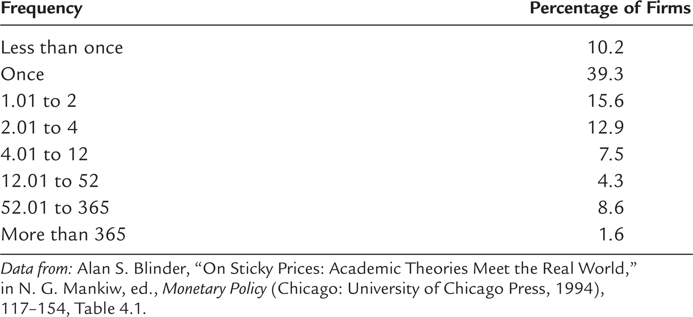
Blinder began by asking firm managers how often they changed prices. The answers, summarized in Table 10-1, yielded two conclusions. First, sticky prices are common. The typical firm in the economy adjusts its prices once or twice a year. Second, there are large differences among firms in the frequency of price adjustment. About 10 percent of firms changed prices more often than once a week, and about the same number changed prices less often than once a year.
TABLE 10-1
TABLE 10-1: The Frequency of Price Adjustment This table is based on answers to the question: How often do the prices of your most important products change in a typical year?

291
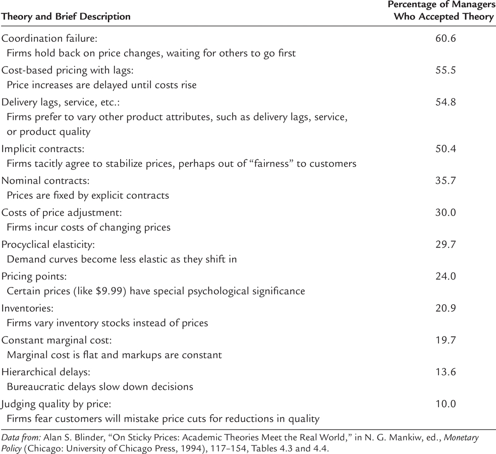
Blinder then asked the firm managers why they didn’t change prices more often. In particular, he explained to the managers several economic theories of sticky prices and asked them to judge how well each of these theories described their firms. Table 10-2 summarizes the theories and ranks them by the percentage of managers who accepted the theory as an accurate description of their firms’ pricing decisions. Notice that each of the theories was endorsed by some of the managers, but each was rejected by a large number as well. One interpretation is that different theories apply to different firms, depending on industry characteristics, and that price stickiness is a macroeconomic phenomenon without a single microeconomic explanation.
TABLE 10-2
TABLE 10-2: Theories of Price Stickiness

292
Among the dozen theories, coordination failure tops the list. According to Blinder, this is an important finding because it suggests that the inability of firms to coordinate price changes plays a key role in explaining price stickiness and, thus, short-run economic fluctuations. He writes, “The most obvious policy implication of the model is that more coordinated wage and price setting—somehow achieved—could improve welfare. But if this proves difficult or impossible, the door is opened to activist monetary policy to cure recessions.”3 
The Model of Aggregate Supply and Aggregate Demand
How does the introduction of sticky prices change our view of how the economy works? We can answer this question by considering economists’ two favorite words—supply and demand.
In classical macroeconomic theory, the amount of output depends on the economy’s ability to supply goods and services, which in turn depends on the supplies of capital and labor and on the available production technology. This is the essence of the basic classical model in Chapter 3, as well as of the Solow growth model in Chapter 8 and Chapter 9. Flexible prices are a crucial assumption of classical theory. The theory posits, sometimes implicitly, that prices adjust to ensure that the quantity of output demanded equals the quantity supplied.
The economy works quite differently when prices are sticky. In this case, as we will see, output also depends on the economy’s demand for goods and services. Demand, in turn, depends on a variety of factors: consumers’ confidence about their economic prospects, firms’ perceptions about the profitability of new investments, and monetary and fiscal policy. Because monetary and fiscal policy can influence demand, and demand in turn can influence the economy’s output over the time horizon when prices are sticky, price stickiness provides a rationale for why these policies may be useful in stabilizing the economy in the short run.
In the rest of this chapter, we begin developing a model that makes these ideas more precise. The place to start is the model of supply and demand, which we used in Chapter 1 to discuss the market for pizza. This basic model offers some of the most fundamental insights in economics. It shows how the supply and demand for any good jointly determine the good’s price and the quantity sold, as well as how shifts in supply and demand affect the price and quantity. We now introduce the “economy-size” version of this model—the model of aggregate supply and aggregate demand. This macroeconomic model allows us to study how the aggregate price level and the quantity of aggregate output are determined in the short run. It also provides a way to contrast how the economy behaves in the long run and how it behaves in the short run.
293
Although the model of aggregate supply and aggregate demand resembles the model of supply and demand for a single good, the analogy is not exact. The model of supply and demand for a single good considers only one good within a large economy. By contrast, as we will see in the coming chapters, the model of aggregate supply and aggregate demand is a sophisticated model that incorporates the interactions among many markets. In the remainder of this chapter we get a first glimpse at those interactions by examining the model in its most simplified form. Our goal here is not to explain the model fully but, instead, to introduce its key elements and illustrate how it can help explain short-run economic fluctuations.