10-4 Aggregate Supply
By itself, the aggregate demand curve does not tell us the price level or the amount of output that will prevail in the economy; it merely gives a relationship between these two variables. To accompany the aggregate demand curve, we need another relationship between P and Y that crosses the aggregate demand curve—an aggregate supply curve. The aggregate demand and aggregate supply curves together pin down the economy’s price level and quantity of output.
Aggregate supply (AS) is the relationship between the quantity of goods and services supplied and the price level. Because the firms that supply goods and services have flexible prices in the long run but sticky prices in the short run, the aggregate supply relationship depends on the time horizon. We need to discuss two different aggregate supply curves: the long-run aggregate supply curve LRAS and the short-run aggregate supply curve SRAS. We also need to discuss how the economy makes the transition from the short run to the long run.
The Long Run: The Vertical Aggregate Supply Curve
Because the classical model describes how the economy behaves in the long run, we derive the long-run aggregate supply curve from the classical model. Recall from Chapter 3 that the amount of output produced depends on the fixed amounts of capital and labor and on the available technology. To show this, we write

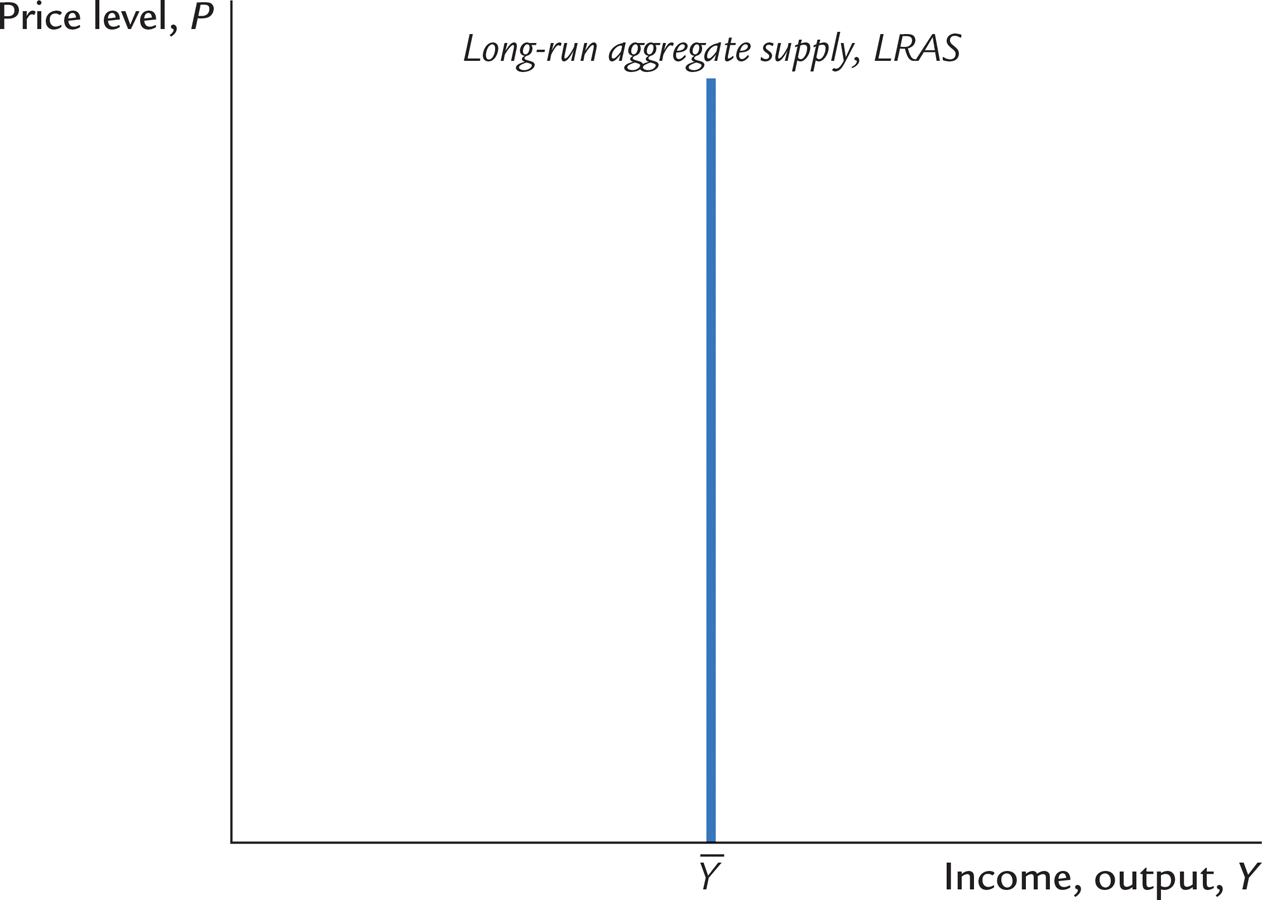
According to the classical model, output does not depend on the price level. To show that output is fixed at this level, regardless of the price level, we draw a vertical aggregate supply curve, as in Figure 10-7. In the long run, the intersection of the aggregate demand curve with this vertical aggregate supply curve determines the price level.
FIGURE 10-7
If the aggregate supply curve is vertical, then changes in aggregate demand affect prices but not output. For example, if the money supply falls, the aggregate demand curve shifts downward, as in Figure 10-8. The economy moves from the old intersection of aggregate supply and aggregate demand, point A, to the new intersection, point B. The shift in aggregate demand affects only prices.
FIGURE 10-8
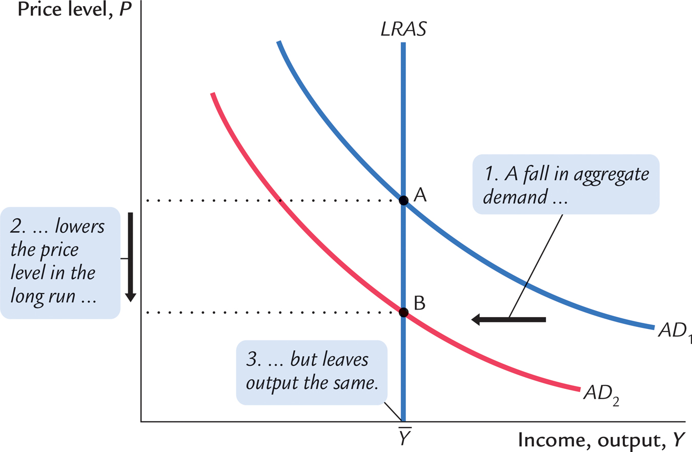
The vertical aggregate supply curve satisfies the classical dichotomy because it implies that the level of output is independent of the money supply. This long-run level of output,  , is called the full-employment, or natural, level of output. It is the level of output at which the economy’s resources are fully employed or, more realistically, at which unemployment is at its natural rate.
The Short Run: The Horizontal Aggregate Supply Curve
The classical model and the vertical aggregate supply curve apply only in the long run. In the short run, some prices are sticky and therefore do not adjust to changes in demand. Because of this price stickiness, the short-run aggregate supply curve is not vertical.
297
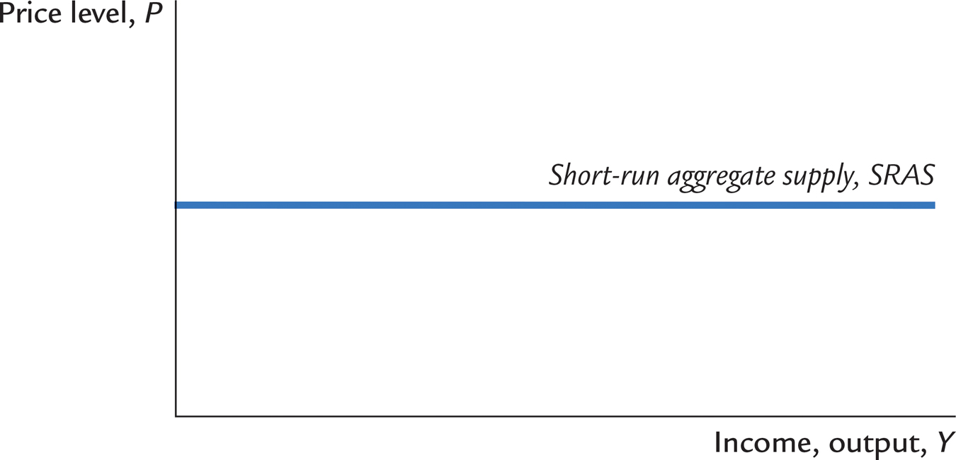
In this chapter, we will simplify things by assuming an extreme example. Suppose that all firms have issued price catalogs and that it is too costly for them to issue new ones. Thus, all prices are stuck at predetermined levels. At these prices, firms are willing to sell as much as their customers are willing to buy, and they hire just enough labor to produce the amount demanded. Because the price level is fixed, we represent this situation in Figure 10-9 with a horizontal aggregate supply curve.
FIGURE 10-9
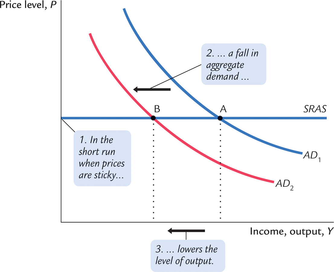
The short-run equilibrium of the economy is the intersection of the aggregate demand curve and this horizontal short-run aggregate supply curve. In this case, changes in aggregate demand do affect the level of output. For example, if the Fed suddenly reduces the money supply, the aggregate demand curve shifts inward, as in Figure 10-10. The economy moves from the old intersection of aggregate demand and aggregate supply, point A, to the new intersection, point B. The movement from point A to point B represents a decline in output at a fixed price level.
FIGURE 10-10
298
Thus, a fall in aggregate demand reduces output in the short run because prices do not adjust instantly. After the sudden fall in aggregate demand, firms are stuck with prices that are too high. With demand low and prices high, firms sell less of their product, so they reduce production and lay off workers. The economy experiences a recession.
Once again, be forewarned that reality is a bit more complicated than illustrated here. Although many prices are sticky in the short run, some prices are able to respond quickly to changing circumstances. As we will see in Chapter 14, in an economy with some sticky prices and some flexible prices, the short-run aggregate supply curve is upward sloping rather than horizontal. Figure 10-10 illustrates the extreme case in which all prices are stuck. Because this case is simpler, it is a useful starting point for thinking about short-run aggregate supply.
299
From the Short Run to the Long Run
We can summarize our analysis so far as follows: Over long periods of time, prices are flexible, the aggregate supply curve is vertical, and changes in aggregate demand affect the price level but not output. Over short periods of time, prices are sticky, the aggregate supply curve is flat, and changes in aggregate demand do affect the economy’s output of goods and services.
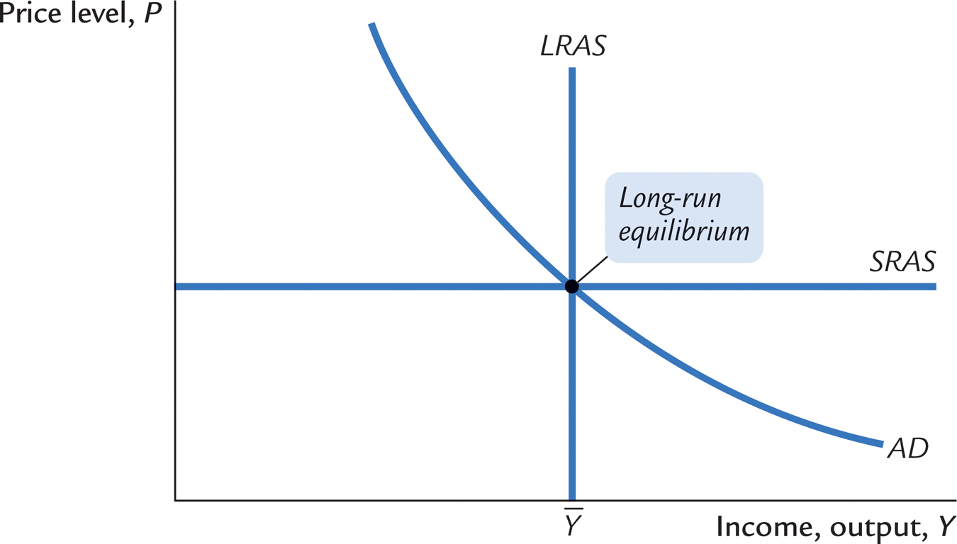
How does the economy make the transition from the short run to the long run? Let’s trace the effects over time of a fall in aggregate demand. Suppose that the economy is initially in long-run equilibrium, as shown in Figure 10-11. In this figure, there are three curves: the aggregate demand curve, the long-run aggregate supply curve, and the short-run aggregate supply curve. The long-run equilibrium is the point at which aggregate demand crosses the long-run aggregate supply curve. Prices have adjusted to reach this equilibrium. Therefore, when the economy is in its long-run equilibrium, the short-run aggregate supply curve must cross this point as well.
FIGURE 10-11
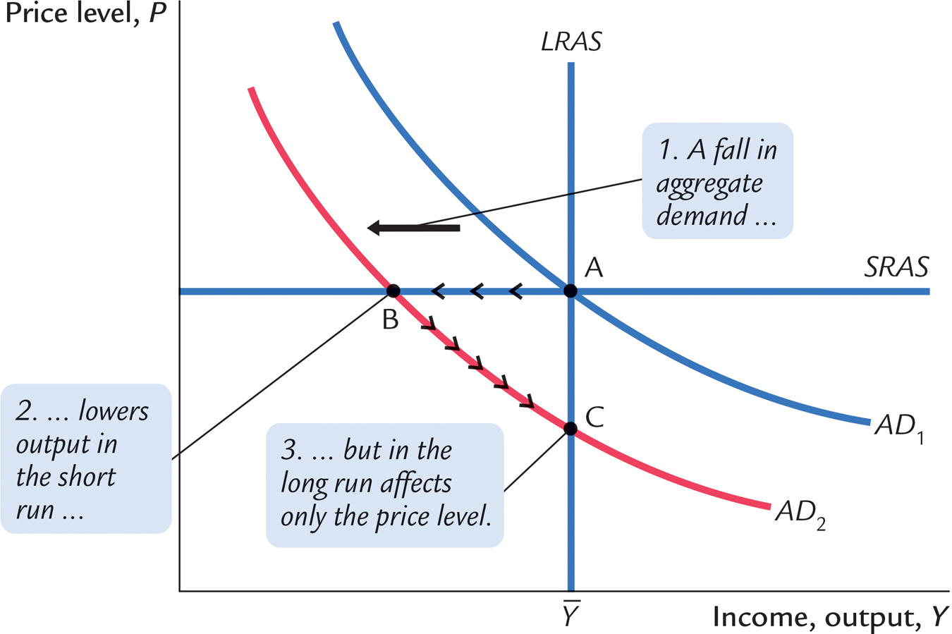
Now suppose that the Fed reduces the money supply and the aggregate demand curve shifts downward, as in Figure 10-12. In the short run, prices are sticky, so the economy moves from point A to point B. Output and employment fall below their natural levels, which means the economy is in a recession. Over time, in response to the low demand, wages and prices fall. The gradual reduction in the price level moves the economy downward along the aggregate demand curve to point C, which is the new long-run equilibrium. In the new long-run equilibrium (point C), output and employment are back to their natural levels, but prices are lower than in the old long-run equilibrium (point A). Thus, a shift in aggregate demand affects output in the short run, but this effect dissipates over time as firms adjust their prices.
FIGURE 10-12
300
CASE STUDY
A Monetary Lesson From French History
Finding modern examples to illustrate the lessons from Figure 10-12 is hard. Modern central banks are too smart to engineer a substantial reduction in the money supply for no good reason. They know that a recession would ensue, and they usually do their best to prevent that from happening. Fortunately, history often fills in the gap when recent experience fails to produce the right experiment.
A vivid example of the effects of monetary contraction occurred in eighteenth-century France. In 2009, François Velde, an economist at the Federal Reserve Bank of Chicago, studied this episode in French economic history.
The story begins with the unusual nature of French money at the time. The money stock in this economy included a variety of gold and silver coins that, in contrast to modern money, did not indicate a specific monetary value. Instead, the monetary value of each coin was set by government decree, and the government could easily change the monetary value and thus the money supply. Sometimes this would occur literally overnight. It is almost as if, while you were sleeping, every $1 bill in your wallet was replaced by a bill worth only 80 cents.
Indeed, that is what happened on September 22, 1724. Every person in France woke up with 20 percent less money than he or she had the night before. Over the course of seven months, the nominal value of the money stock was reduced by about 45 percent. The goal of these changes was to reduce prices in the economy to what the government considered an appropriate level.
What happened as a result of this policy? Velde reports the following consequences:
Although prices and wages did fall, they did not do so by the full 45 percent; moreover, it took them months, if not years, to fall that far. Real wages in fact rose, at least initially. Interest rates rose. The only market that adjusted instantaneously and fully was the foreign exchange market. Even markets that were as close to fully competitive as one can imagine, such as grain markets, failed to react initially….
301
At the same time, the industrial sector of the economy (or at any rate the textile industry) went into a severe contraction, by about 30 percent. The onset of the recession may have occurred before the deflationary policy began, but it was widely believed at the time that the severity of the contraction was due to monetary policy, in particular to a resulting “credit crunch” as holders of money stopped providing credit to trade in anticipation of further price declines (the “scarcity of money” frequently blamed by observers). Likewise, it was widely believed (on the basis of past experience) that a policy of inflation would halt the recession, and coincidentally or not, the economy rebounded once the nominal money supply was increased by 20 percent in May 1726.
This description of events from French history fits well with the lessons from mainstream macroeconomic theory.4 
FYI
David Hume on the Real Effects of Money
As noted in Chapter 5, many of the central ideas of monetary theory have a long history. The classical theory of money we discussed in that chapter dates back as far as the eighteenth-century philosopher and economist David Hume. While Hume understood that changes in the money supply ultimately led to inflation, he also knew that money had real effects in the short run. Here is how Hume described a monetary injection in his 1752 essay Of Money:
To account, then, for this phenomenon, we must consider, that though the high price of commodities be a necessary consequence of the increase of gold and silver, yet it follows not immediately upon that increase; but some time is required before the money circulates through the whole state, and makes its effect be felt on all ranks of people. At first, no alteration is perceived; by degrees the price rises, first of one commodity, then of another; till the whole at last reaches a just proportion with the new quantity of specie which is in the kingdom. In my opinion, it is only in this interval or intermediate situation, between the acquisition of money and rise of prices, that the increasing quantity of gold and silver is favorable to industry. When any quantity of money is imported into a nation, it is not at first dispersed into many hands; but is confined to the coffers of a few persons, who immediately seek to employ it to advantage. Here are a set of manufacturers or merchants, we shall suppose, who have received returns of gold and silver for goods which they sent to Cadiz. They are thereby enabled to employ more workmen than formerly, who never dream of demanding higher wages, but are glad of employment from such good paymasters. If workmen become scarce, the manufacturer gives higher wages, but at first requires an increase of labor; and this is willingly submitted to by the artisan, who can now eat and drink better, to compensate his additional toil and fatigue. He carries his money to market, where he finds everything at the same price as formerly, but returns with greater quantity and of better kinds, for the use of his family. The farmer and gardener, finding that all their commodities are taken off, apply themselves with alacrity to the raising more; and at the same time can afford to take better and more cloths from their tradesmen, whose price is the same as formerly, and their industry only whetted by so much new gain. It is easy to trace the money in its progress through the whole commonwealth; where we shall find, that it must first quicken the diligence of every individual, before it increases the price of labor.
Though written more than two centuries ago, these words reflect well the modern understanding of the short-run effects of changes in the money supply.
302