11-1 The Goods Market and the IS Curve
The IS curve plots the relationship between the interest rate and the level of income that arises in the market for goods and services. To develop this relationship, we start with a basic model called the Keynesian cross. This model is the simplest interpretation of Keynes’s theory of how national income is determined and is a building block for the more complex and realistic IS–LM model.
The Keynesian Cross
In The General Theory, Keynes proposed that an economy’s total income is, in the short run, determined largely by the spending plans of households, businesses, and government. The more people want to spend, the more goods and services firms can sell. The more firms can sell, the more output they will choose to produce and the more workers they will choose to hire. Keynes believed that the problem during recessions and depressions is inadequate spending. The Keynesian cross is an attempt to model this insight.
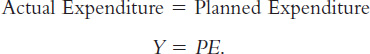
Planned Expenditure We begin our derivation of the Keynesian cross by drawing a distinction between actual and planned expenditure. Actual expenditure is the amount households, firms, and the government spend on goods and services, and as we first saw in Chapter 2, it equals the economy’s gross domestic product (GDP). Planned expenditure is the amount households, firms, and the government would like to spend on goods and services.
Why would actual expenditure ever differ from planned expenditure? The answer is that firms might engage in unplanned inventory investment because their sales do not meet their expectations. When firms sell less of their product than they planned, their stock of inventories automatically rises; conversely, when firms sell more than planned, their stock of inventories falls. Because these unplanned changes in inventory are counted as investment spending by firms, actual expenditure can be either above or below planned expenditure.
314
Now consider the determinants of planned expenditure. Assuming that the economy is closed, so that net exports are zero, we write planned expenditure PE as the sum of consumption C, planned investment I, and government purchases G:
PE = C + I + G.
To this equation, we add the consumption function:
C = C(Y − T).
This equation states that consumption depends on disposable income (Y − T), which is total income Y minus taxes T. To keep things simple, for now we take planned investment as exogenously fixed:

Finally, as in Chapter 3, we assume that fiscal policy—

Combining these five equations, we obtain

This equation shows that planned expenditure is a function of income Y, the level of planned investment  , and the fiscal policy variables
  and
and  .
.
Figure 11-2 graphs planned expenditure as a function of the level of income. This line slopes upward because higher income leads to higher consumption and thus higher planned expenditure. The slope of this line is the marginal propensity to consume, MPC: it shows how much planned expenditure increases when income rises by $1. This planned-
FIGURE 11-2

315
The Economy in Equilibrium The next piece of the Keynesian cross is the assumption that the economy is in equilibrium when actual expenditure equals planned expenditure. This assumption is based on the idea that when people’s plans have been realized, they have no reason to change what they are doing. Recalling that Y as GDP equals not only total income but also total actual expenditure on goods and services, we can write this equilibrium condition as
The 45-
FIGURE 11-3

How does the economy get to equilibrium? In this model, inventories play an important role in the adjustment process. Whenever an economy is not in equilibrium, firms experience unplanned changes in inventories, and this induces them to change production levels. Changes in production in turn influence total income and expenditure, moving the economy toward equilibrium.
For example, suppose the economy finds itself with GDP at a level greater than the equilibrium level, such as the level Y1 in Figure 11-4. In this case, planned expenditure PE1 is less than production Y1, so firms are selling less than they are producing. Firms add the unsold goods to their stock of inventories. This unplanned rise in inventories induces firms to lay off workers and reduce production; these actions in turn reduce GDP. This process of unintended inventory accumulation and falling income continues until income Y falls to the equilibrium level.
FIGURE 11-4

316
Similarly, suppose GDP is at a level lower than the equilibrium level, such as the level Y2 in Figure 11-4. In this case, planned expenditure PE2 is greater than production Y2. Firms meet the high level of sales by drawing down their inventories. But when firms see their stock of inventories dwindle, they hire more workers and increase production. GDP rises, and the economy approaches equilibrium.
In summary, the Keynesian cross shows how income Y is determined for given levels of planned investment I and fiscal policy G and T. We can use this model to show how income changes when one of these exogenous variables changes.
Fiscal Policy and the Multiplier: Government Purchases Consider how changes in government purchases affect the economy. Because government purchases are one component of expenditure, higher government purchases result in higher planned expenditure for any given level of income. If government purchases rise by ΔG, then the planned-
FIGURE 11-5

This graph shows that an increase in government purchases leads to an even greater increase in income. That is, ΔY is larger than ΔG. The ratio ΔY/ΔG is called the government-
317
Why does fiscal policy have a multiplied effect on income? The reason is that, according to the consumption function C = C(Y − T), higher income causes higher consumption. When an increase in government purchases raises income, it also raises consumption, which further raises income, which further raises consumption, and so on. Therefore, in this model, an increase in government purchases causes a greater increase in income.
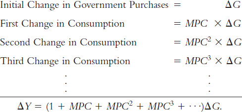
How big is the multiplier? To answer this question, we trace through each step of the change in income. The process begins when expenditure rises by ΔG, which implies that income rises by ΔG as well. This increase in income in turn raises consumption by MPC × ΔG, where MPC is the marginal propensity to consume. This increase in consumption raises expenditure and income once again. This second increase in income of MPC × ΔG again raises consumption, this time by MPC × (MPC × ΔG), which again raises expenditure and income, and so on. This feedback from consumption to income to consumption continues indefinitely. The total effect on income is
318
The government-
ΔY/ΔG = 1 + MPC + MPC2 + MPC3 + ….
This expression for the multiplier is an example of an infinite geometric series. A result from algebra allows us to write the multiplier as2
ΔY/ΔG = 1/(1 − MPC).
For example, if the marginal propensity to consume is 0.6, the multiplier is
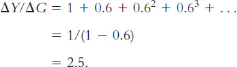
In this case, a $1.00 increase in government purchases raises equilibrium income by $2.50.3
Fiscal Policy and the Multiplier: Taxes Now consider how changes in taxes affect equilibrium income. A decrease in taxes of ΔT immediately raises disposable income Y − T by ΔT and, therefore, increases consumption by MPC × ΔT. For any given level of income Y, planned expenditure is now higher. As Figure 11-6 shows, the planned-
FIGURE 11-6

319
Just as an increase in government purchases has a multiplied effect on income, so does a decrease in taxes. As before, the initial change in expenditure, now MPC × ΔT, is multiplied by 1/(1 − MPC). The overall effect on income of the change in taxes is
ΔY/ΔT = −MPC/(1 − MPC).
This expression is the tax multiplier, the amount income changes in response to a $1 change in taxes. (The negative sign indicates that income moves in the opposite direction from taxes.) For example, if the marginal propensity to consume is 0.6, then the tax multiplier is
ΔY/ΔT = −0.6/(1 − 0.6) = −1.5.
In this example, a $1.00 cut in taxes raises equilibrium income by $1.50.4
320
CASE STUDY
Cutting Taxes to Stimulate the Economy: The Kennedy and Bush Tax Cuts
When John F. Kennedy became president of the United States in 1961, he brought to Washington some of the brightest young economists of the day to work on his Council of Economic Advisers. These economists, who had been schooled in the economics of Keynes, brought Keynesian ideas to discussions of economic policy at the highest level.
One of the council’s first proposals was to expand national income by reducing taxes. This eventually led to a substantial cut in personal and corporate income taxes in 1964. The tax cut was intended to stimulate expenditure on consumption and investment and thus lead to higher levels of income and employment. When a reporter asked Kennedy why he advocated a tax cut, Kennedy replied, “To stimulate the economy. Don’t you remember your Economics 101?”
As Kennedy’s economic advisers predicted, the passage of the tax cut was followed by an economic boom. Growth in real GDP was 5.8 percent in 1964 and 6.5 percent in 1965. The unemployment rate fell from 5.6 percent in 1963 to 5.2 percent in 1964 and then to 4.5 percent in 1965.
Economists continue to debate the source of this rapid growth in the early 1960s. A group called supply-
When George W. Bush was elected president in 2000, a major element of his platform was a cut in income taxes. Bush and his advisers used both supply-
Congress passed major tax cuts in 2001 and 2003. After the second tax cut, the weak recovery from the 2001 recession turned into a more robust one. Growth in real GDP was 3.8 percent in 2004. The unemployment rate fell from its peak of 6.3 percent in June 2003 to 4.9 percent in December 2005.
When President Bush signed the 2003 tax bill, he explained the measure using the logic of aggregate demand: “When people have more money, they can spend it on goods and services. And in our society, when they demand an additional good or a service, somebody will produce the good or a service. And when somebody produces that good or a service, it means somebody is more likely to be able to find a job.” The explanation could have come from an exam in Economics 101. 
321
CASE STUDY
Increasing Government Purchases to Stimulate the Economy: The Obama Stimulus
When President Barack Obama took office in January 2009, the economy was suffering from a significant recession. (The causes of this recession are discussed in a Case Study in the next chapter and in more detail in Chapter 20.) Even before he was inaugurated, the president and his advisers proposed a sizable stimulus package to increase aggregate demand. As proposed, the package would cost the federal government about $800 billion, or about 5 percent of annual GDP. The package included some tax cuts and higher transfer payments, but much of it was made up of increases in government purchases of goods and services.

Professional economists debated the merits of the plan. Advocates of the Obama plan argued that increased spending was better than reduced taxes because, according to standard Keynesian theory, the government-
The Obama stimulus proposal was controversial among economists for various reasons. One criticism was that the stimulus was not large enough given the apparent depth of the economic downturn. In March 2009, economist Paul Krugman wrote in the New York Times:
The plan was too small and too cautious…. Employment has already fallen more in this recession than in the 1981–
322
Still other economists argued that despite the predictions of conventional Keynesian models, spending-
In addition, some economists thought that using infrastructure spending to promote employment might conflict with the goal of obtaining the infrastructure that was most needed. Here is how economist Gary Becker explained the concern on his blog:
Putting new infrastructure spending in depressed areas like Detroit might have a big stimulating effect since infrastructure building projects in these areas can utilize some of the considerable unemployed resources there. However, many of these areas are also declining because they have been producing goods and services that are not in great demand, and will not be in demand in the future. Therefore, the overall value added by improving their roads and other infrastructure is likely to be a lot less than if the new infrastructure were located in growing areas that might have relatively little unemployment, but do have great demand for more roads, schools, and other types of long-
In the end, Congress went ahead with President Obama’s proposed stimulus plans with relatively minor modifications. The president signed the $787 billion bill on February 17, 2009. Did it work? The economy recovered from the recession, but more slowly than the Obama administration economists initially forecast. Whether the slow recovery reflects the failure of stimulus policy or a sicker economy than the economists first appreciated is a question of continuing debate.
CASE STUDY
Using Regional Data to Estimate Multipliers
As the preceding two case studies show, policymakers often change taxes and government spending to influence the economy. The short-
Unfortunately, that question is hard to answer. When policymakers change fiscal policy, they usually do so for good reason. Because many other things are happening at the same time, there is no easy way to separate the effects of the fiscal policy from the effects of the other events. For example, President Obama proposed his 2009 stimulus plan because the economy was suffering in the aftermath of a financial crisis. We can observe what happened to the economy after the stimulus was passed, but disentangling the effects of the stimulus from the lingering effects of the financial crisis is a formidable task.
323
Increasingly, economists have tried to estimate multipliers for fiscal policy using regional data from states or provinces within a country. The use of regional data has two advantages. First, it increases the number of observations: the United States, for instance, has only one national economy but 50 state economies. Second, and more important, it is possible to find variation in regional government spending that is plausibly unrelated to other events affecting the regional economy. By examining such random variation in government spending, a researcher can more easily identify its macroeconomic effects without being led astray by other, confounding variables.
In one such study, Emi Nakamura and Jón Steinsson looked at the impact of defense spending on state economies. They began with the fact that states vary considerably in the size of their defense industries. For example, military contractors are more important in California than in Illinois: when the U.S. federal government increases defense spending by 1% of U.S. GDP, defense spending in California rises on average by about 3% of California GDP, while defense spending in Illinois rises by only about 0.5% of Illinois GDP. By examining what happens to the California economy relative to the Illinois economy when the United States embarks on a military buildup, we can estimate the effects of government spending. Using data from all 50 states, Nakamura and Steinsson reported a government-
In another study, Antonio Acconcia, Giancarlo Corsetti, and Saverio Simonelli used data from provinces within Italy to study the multiplier. Here the variation in government spending comes not from military buildups but from an Italian law cracking down on organized crime. According to the law, whenever the police uncover incriminating evidence that the Mafia has infiltrated a city council, the council is dismissed and replaced by external commissioners. These commissioners typically implement an immediate, unanticipated, and temporary cut in public investment projects. The study reported that this cut in government spending has a significant impact on the province’s GDP. Once again, the multiplier is estimated to be about 1.5. Hence, these studies confirm the prediction of Keynesian theory that changes in government purchases can have a sizeable effect on an economy’s output of goods and services.
It is unclear, however, how to use these estimates from regional economies to draw inferences about national economies. One problem is that the regional government spending these researchers studied was not financed with regional taxes. Defense spending in California is largely paid for by federal taxes levied on the other 49 states, and the public investment projects in an Italian province are largely paid for at the national level. By contrast, when a nation increases its government spending, it has to increase taxes, either in the present or the future, to pay for it. These higher taxes could depress economic activity, leading to a smaller multiplier. A second problem is that these regional changes in government spending do not influence monetary policy, because central banks focus on national rather than regional conditions. By contrast, a national change in government spending could well induce a change in monetary policy. In its attempt to stabilize the economy, the central bank may offset some of the effects of fiscal policy, making the multiplier smaller.
324
Although both of these problems suggest that national multipliers are likely smaller than regional multipliers, a third problem works in the opposite direction. In a small regional economy, such as a state, many of the goods and services people buy are imported from neighboring states, whereas imports are a smaller share of a large national economy. When imports play a larger role, the marginal propensity to consume on domestic goods (those made within the state) is smaller. As the Keynesian cross describes, a smaller marginal propensity to consume on domestic goods leads to smaller second-
The bottom line from studies of regional economies is that the demand from government purchases can exert a strong influence on economic activity. But the size of that effect as measured by the multiplier at the national level remains open to debate.7
The Interest Rate, Investment, and the IS Curve
The Keynesian cross is only a stepping-
To add this relationship between the interest rate and investment to our model, we write the level of planned investment as
I = I(r).
This investment function is graphed in panel (a) of Figure 11-7. Because the interest rate is the cost of borrowing to finance investment projects, an increase in the interest rate reduces planned investment. As a result, the investment function slopes downward.
FIGURE 11-7

325
To determine how income changes when the interest rate changes, we can combine the investment function with the Keynesian-
The IS curve, shown in panel (c) of Figure 11-7, summarizes this relationship between the interest rate and the level of income. In essence, the IS curve combines the interaction between r and I expressed by the investment function and the interaction between I and Y demonstrated by the Keynesian cross. Each point on the IS curve represents equilibrium in the goods market, and the curve illustrates how the equilibrium level of income depends on the interest rate. Because an increase in the interest rate causes planned investment to fall, which in turn causes equilibrium income to fall, the IS curve slopes downward.
326
How Fiscal Policy Shifts the IS Curve
The IS curve shows us, for any given interest rate, the level of income that brings the goods market into equilibrium. As we learned from the Keynesian cross, the equilibrium level of income also depends on government spending G and taxes T. The IS curve is drawn for a given fiscal policy; that is, when we construct the IS curve, we hold G and T fixed. When fiscal policy changes, the IS curve shifts.
Figure 11-8 uses the Keynesian cross to show how an increase in government purchases ΔG shifts the IS curve. This figure is drawn for a given interest rate  and thus for a given level of planned investment. The Keynesian cross in panel (a) shows that this change in fiscal policy raises planned expenditure and thereby increases equilibrium income from Y1 to Y2. Therefore, in panel (b), the increase in government purchases shifts the IS curve outward.
FIGURE 11-8

327
We can use the Keynesian cross to see how other changes in fiscal policy shift the IS curve. Because a decrease in taxes also expands expenditure and income, it, too, shifts the IS curve outward. A decrease in government purchases or an increase in taxes reduces income; therefore, such a change in fiscal policy shifts the IS curve inward.
In summary, the IS curve shows the combinations of the interest rate and the level of income that are consistent with equilibrium in the market for goods and services. The IS curve is drawn for a given fiscal policy. Changes in fiscal policy that raise the demand for goods and services shift the IS curve to the right. Changes in fiscal policy that reduce the demand for goods and services shift the IS curve to the left.