Now that we have developed the model of aggregate demand, let’s use it to address the question that originally motivated Keynes: what caused the Great Depression? Even today, almost a century after the event, economists continue to debate the cause of this major economic downturn. The Great Depression provides an extended case study to show how economists use the IS–LM model to analyze economic fluctuations.1

Before turning to the explanations economists have proposed, look at Table 12-1, which presents some statistics regarding the Depression. These statistics are the battlefield on which debate about the Depression takes place. What do you think happened? An IS shift? An LM shift? Or something else?

Table 12-1 shows that the decline in income in the early 1930s coincided with falling interest rates. This fact has led some economists to suggest that the cause of the decline may have been a contractionary shift in the IS curve. This view is sometimes called the spending hypothesis because it places primary blame for the Depression on an exogenous fall in spending on goods and services.

Economists have attempted to explain this decline in spending in several ways. Some argue that a downward shift in the consumption function caused the contractionary shift in the IS curve. The stock market crash of 1929 may have been partly responsible for this shift: by reducing wealth and increasing uncertainty about the future prospects of the U.S. economy, the crash may have induced consumers to save more of their income rather than spend it.

Others explain the decline in spending by pointing to the large drop in investment in housing. Some economists believe that the residential investment boom of the 1920s was excessive and that once this “overbuilding” became apparent, the demand for residential investment declined drastically. Another possible explanation for the fall in residential investment is the reduction in immigration in the 1930s: a more slowly growing population demands less new housing.

352

Once the Depression began, several events occurred that could have reduced spending further. First, many banks failed in the early 1930s, in part because of inadequate bank regulation, and these bank failures may have exacerbated the fall in investment spending. Banks play the crucial role of getting the funds available for investment to those households and firms that can best use them. The closing of many banks in the early 1930s may have prevented some businesses from getting the funds they needed for capital investment and, therefore, may have led to a further contraction in investment spending.2

The fiscal policy of the 1930s also contributed to the contractionary shift in the IS curve. Politicians at that time were more concerned with balancing the budget than with using fiscal policy to keep production and employment at their natural levels. The Revenue Act of 1932 increased various taxes, especially those falling on lower- and middle-income consumers.3 The Democratic platform of that year expressed concern about the budget deficit and advocated an “immediate and drastic reduction of governmental expenditures.” In the midst of historically high unemployment, policymakers searched for ways to raise taxes and reduce government spending.

353

There are, therefore, several ways to explain a contractionary shift in the IS curve. Keep in mind that these different views may all be true. There may be no single explanation for the decline in spending. It is possible that all of these changes coincided and that together they led to a massive reduction in spending.

Table 12-1 shows that the money supply fell 25 percent from 1929 to 1933, during which time the unemployment rate rose from 3.2 percent to 25.2 percent. This fact provides the motivation and support for what is called the money hypothesis, which places primary blame for the Depression on the Federal Reserve for allowing the money supply to fall by such a large amount.4 The best-known advocates of this interpretation are Milton Friedman and Anna Schwartz, who defended it in their treatise on U.S. monetary history. Friedman and Schwartz argue that contractions in the money supply have caused most economic downturns and that the Great Depression is a particularly vivid example.

354

Using the IS–LM model, we might interpret the money hypothesis as explaining the Depression by a contractionary shift in the LM curve. Seen in this way, however, the money hypothesis runs into two problems.

The first problem is the behavior of real money balances. Monetary policy leads to a contractionary shift in the LM curve only if real money balances fall. Yet from 1929 to 1931 real money balances rose slightly because the fall in the money supply was accompanied by an even greater fall in the price level. Although the monetary contraction may have been responsible for the rise in unemployment from 1931 to 1933, when real money balances did fall, it cannot easily explain the initial downturn from 1929 to 1931.

The second problem for the money hypothesis is the behavior of interest rates. If a contractionary shift in the LM curve triggered the Depression, we should have observed higher interest rates. Yet nominal interest rates fell continuously from 1929 to 1933.

These two reasons appear sufficient to reject the view that the Depression was instigated by a contractionary shift in the LM curve. But was the fall in the money stock irrelevant? Next, we turn to another mechanism through which monetary policy might have been responsible for the severity of the Depression—the deflation of the 1930s.

From 1929 to 1933 the price level fell 22 percent. Many economists blame this deflation for the severity of the Great Depression. They argue that the deflation may have turned what in 1931 was a typical economic downturn into an unprecedented period of high unemployment and depressed income. If correct, this argument gives new life to the money hypothesis. Because the falling money supply was, plausibly, responsible for the falling price level, it could have been responsible for the severity of the Depression. To evaluate this argument, we must discuss how changes in the price level affect income in the IS–LM model.

The Stabilizing Effects of Deflation In the IS–LM model we have developed so far, falling prices raise income. For any given supply of money M, a lower price level implies higher real money balances M/P. An increase in real money balances causes an expansionary shift in the LM curve, which leads to higher income.

Another channel through which falling prices expand income is called the Pigou effect. Arthur Pigou, a prominent classical economist in the 1930s, pointed out that real money balances are part of households’ wealth. As prices fall and real money balances rise, consumers should feel wealthier and spend more. This increase in consumer spending should cause an expansionary shift in the IS curve, also leading to higher income.

These two reasons led some economists in the 1930s to believe that falling prices would help stabilize the economy. That is, they thought that a decline in the price level would automatically push the economy back toward full employment. Yet other economists were less confident in the economy’s ability to correct itself. They pointed to other effects of falling prices, to which we now turn.

355

The Destabilizing Effects of Deflation Economists have proposed two theories to explain how falling prices could depress income rather than raise it. The first, called the debt-deflation theory, describes the effects of unexpected falls in the price level. The second explains the effects of expected deflation.

The debt-deflation theory begins with an observation from Chapter 5: unanticipated changes in the price level redistribute wealth between debtors and creditors. If a debtor owes a creditor $1,000, then the real amount of this debt is $1,000/P, where P is the price level. A fall in the price level raises the real amount of this debt—the amount of purchasing power the debtor must repay the creditor. Therefore, an unexpected deflation enriches creditors and impoverishes debtors.

The debt-deflation theory then posits that this redistribution of wealth affects spending on goods and services. In response to the redistribution from debtors to creditors, debtors spend less and creditors spend more. If these two groups have equal spending propensities, there is no aggregate impact. But it seems reasonable to assume that debtors have higher propensities to spend than creditors—perhaps that is why the debtors are in debt in the first place. In this case, debtors reduce their spending by more than creditors raise theirs. The net effect is a reduction in spending, a contractionary shift in the IS curve, and lower national income.

To understand how expected changes in prices can affect income, we need to add a new variable to the IS–LM model. Our discussion of the model so far has not distinguished between the nominal and real interest rates. Yet we know from previous chapters that investment depends on the real interest rate and that money demand depends on the nominal interest rate. If i is the nominal interest rate and Eπ is expected inflation, then the ex ante real interest rate is i − Eπ. We can now write the IS–LM model as

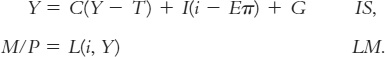
Expected inflation enters as a variable in the IS curve. Thus, changes in expected inflation shift the IS curve.

Let’s use this extended IS–LM model to examine how changes in expected inflation influence the level of income. We begin by assuming that everyone expects the price level to remain the same. In this case, there is no expected inflation (Eπ = 0), and these two equations produce the familiar IS–LM model. Figure 12-8 depicts this initial situation with the LM curve and the IS curve labeled IS₁. The intersection of these two curves determines the nominal and real interest rates, which for now are the same.

Now suppose that everyone suddenly expects that the price level will fall in the future, so that Eπ becomes negative. The real interest rate is now higher at any given nominal interest rate. This increase in the real interest rate depresses planned investment spending, shifting the IS curve from IS₁ to IS₂. (The vertical distance of the downward shift exactly equals the expected deflation.) Thus, an expected deflation leads to a reduction in national income from Y₁ to Y₂. The nominal interest rate falls from i₁ to i₂, while the real interest rate rises from r₁ to r₂.

Here is the story behind this figure. When firms come to expect deflation, they become reluctant to borrow to buy investment goods because they believe they will have to repay these loans later in more valuable dollars. The fall in investment depresses planned expenditure, which in turn depresses income. The fall in income reduces the demand for money, and this reduces the nominal interest rate that equilibrates the money market. The nominal interest rate falls by less than the expected deflation, so the real interest rate rises.

356

Note that there is a common thread in these two stories of destabilizing deflation. In both, falling prices depress national income by causing a contractionary shift in the IS curve. Because a deflation of the size observed from 1929 to 1933 is unlikely except in the presence of a major contraction in the money supply, these two explanations assign some of the responsibility for the Depression—especially its severity—to the Fed. In other words, if falling prices are destabilizing, then a contraction in the money supply can lead to a fall in income, even without a decrease in real money balances or a rise in nominal interest rates.

Economists study the Depression both because of its intrinsic interest as a major economic event and to provide guidance to policymakers so that it will not happen again. To state with confidence whether this event could recur, we would need to know why it happened. Because there is not yet agreement on the causes of the Great Depression, it is impossible to rule out with certainty another depression of this magnitude.

Yet most economists believe that the mistakes that led to the Great Depression are unlikely to be repeated. The Fed seems unlikely to allow the money supply to fall by one-fourth. Many economists believe that the deflation of the early 1930s was responsible for the depth and length of the Depression. And it seems likely that such a prolonged deflation was possible only in the presence of a falling money supply.

357

The fiscal-policy mistakes of the Depression are also unlikely to be repeated. Fiscal policy in the 1930s not only failed to help but actually further depressed aggregate demand. Few economists today would advocate such a rigid adherence to a balanced budget in the face of massive unemployment.

In addition, there are many institutions today that would help prevent the events of the 1930s from recurring. The system of federal deposit insurance makes widespread bank failures less likely. The income tax causes an automatic reduction in taxes when income falls, which stabilizes the economy. Finally, economists know more today than they did in the 1930s. Our knowledge of how the economy works, limited as it still is, should help policymakers formulate better policies to combat such widespread unemployment.

360

In the United States in the 1930s, interest rates reached very low levels. As Table 12-1 shows, U.S. interest rates were well under 1 percent throughout the second half of the 1930s. A similar situation occurred during the economic downturn of 2008–2009. In December 2008, the Federal Reserve cut its target for the federal funds rate to the range of zero to 0.25 percent, and it kept the rate at that level at least until this book was going to press in early 2015.

Some economists describe this situation as a liquidity trap. According to the IS–LM model, expansionary monetary policy works by reducing interest rates and stimulating investment spending. But if interest rates have already fallen almost to zero, then perhaps monetary policy is no longer effective. Nominal interest rates cannot fall below zero: rather than making a loan at a negative nominal interest rate, a person would just hold cash. In this environment, expansionary monetary policy increases the supply of money, making the public’s asset portfolio more liquid, but because interest rates can’t fall any farther, the extra liquidity might not have any effect. Aggregate demand, production, and employment may be “trapped” at low levels. The liquidity trap is sometimes called the problem of the zero lower bound.

Other economists are skeptical about the relevance of liquidity traps and believe that central banks continue to have tools to expand the economy, even after the interest rate target hits the lower bound of zero. One possibility is that a central bank could try to lower longer-term interest rates. It can accomplish this by committing to keep the target interest rate (typically a very short-term interest rate) low for an extended period of time. A policy of announcing future monetary actions is sometimes called forward guidance. A central bank can also lower longer-term interest rates by conducting expansionary open-market operations in a larger variety of financial instruments than it normally does. For example, it could buy long-term government bonds, mortgages, and corporate debt and thereby lower the interest rates on these kinds of loans, a policy sometimes called quantitative easing. During the downturn of 2008–2009 and its aftermath, the Federal Reserve actively pursued a policy of forward guidance and quantitative easing.

Another way that monetary expansion can expand the economy despite the zero lower bound is that it could cause the currency to lose value in the market for foreign-currency exchange. This depreciation would make the nation’s goods cheaper abroad, stimulating export demand. This mechanism goes beyond the closed-economy IS–LM model we have used in this chapter, but it fits well with the open-economy version of the model developed in the next chapter.

Some economists have argued that the possibility of a liquidity trap argues for a target rate of inflation greater than zero. Under zero inflation, the real interest rate, like the nominal interest, can never fall below zero. But if the normal rate of inflation is, say, 4 percent, then the central bank can easily push the real interest rate to negative 4 percent by lowering the nominal interest rate toward zero. Put differently, a higher target for the inflation rate means a higher nominal interest rate in normal times (recall the Fisher effect), which in turn gives the central bank more room to cut interest rates when the economy experiences recessionary shocks. Thus, a higher inflation target gives monetary policymakers more room to stimulate the economy when needed, reducing the likelihood that the economy will hit the zero lower bound and fall into a liquidity trap.5

361