Before analyzing the impact of policies in an open economy, we must specify the international monetary system in which the country has chosen to operate. That is, we must consider how people engaged in international trade and finance can convert the currency of one country into the currency of another.

We start with the system relevant for most major economies today: floating exchange rates. Under a system of floating exchange rates, the exchange rate is set by market forces and is allowed to fluctuate in response to changing economic conditions. In this case, the exchange rate e adjusts to achieve simultaneous equilibrium in the goods market and the money market. When something happens to change that equilibrium, the exchange rate is allowed to move to a new equilibrium value.

Let’s now consider three policies that can change the equilibrium: fiscal policy, monetary policy, and trade policy. Our goal is to use the Mundell–Fleming model to show the effects of policy changes and to understand the economic forces at work as the economy moves from one equilibrium to another.

374

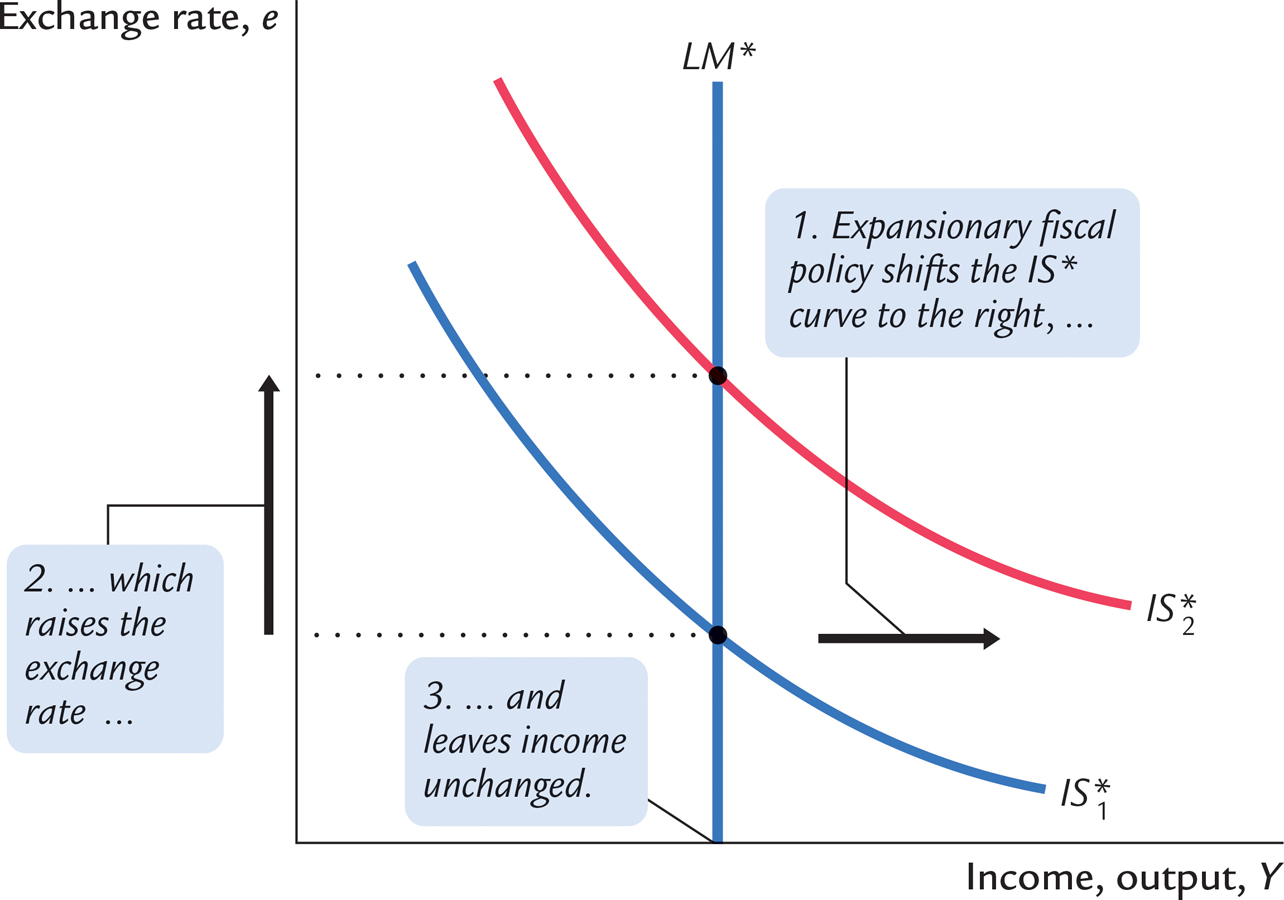
Suppose that the government stimulates domestic spending by increasing government purchases or by cutting taxes. Because such expansionary fiscal policy increases planned expenditure, it shifts the IS* curve to the right, as in Figure 13-4. As a result, the exchange rate appreciates, while the level of income remains the same.

Notice that fiscal policy has very different effects in a small open economy than it does in a closed economy. In the closed-economy IS–LM model, a fiscal expansion raises income, whereas in a small open economy with a floating exchange rate, a fiscal expansion leaves income at the same level. Mechanically, the difference arises because the LM* curve is vertical, while the LM curve we used to study a closed economy is upward sloping. But this explanation is not very satisfying. What are the economic forces that lie behind the different outcomes? To answer this question, we must think through what is happening to the international flow of capital and the implications of these capital flows for the domestic economy.

The interest rate and the exchange rate are the key variables in the story. When income rises in a closed economy, the interest rate rises because higher income increases the demand for money. That is not possible in a small open economy because, as soon as the interest rate starts to rise above the world interest rate r*, capital quickly flows in from abroad to take advantage of the higher return. As this capital inflow pushes the interest rate back to r*, it also has another effect: because foreign investors need to buy the domestic currency to invest in the domestic economy, the capital inflow increases the demand for the domestic currency in the market for foreign-currency exchange, bidding up the value of the domestic currency. The appreciation of the domestic currency makes domestic goods more expensive relative to foreign goods, reducing net exports. The fall in net exports exactly offsets the effects of the expansionary fiscal policy on income.

375

Why is the fall in net exports so great that it renders fiscal policy powerless to influence income? To answer this question, consider the equation that describes the money market:

M/P = L(r, Y).

In both closed and open economies, the quantity of real money balances supplied M/P is fixed by the central bank (which sets M) and the assumption of sticky prices (which fixes P). The quantity demanded (determined by r and Y) must equal this fixed supply. In a closed economy, a fiscal expansion causes the equilibrium interest rate to rise. This increase in the interest rate (which reduces the quantity of money demanded) is accompanied by an increase in equilibrium income (which raises the quantity of money demanded); these two effects together maintain equilibrium in the money market. By contrast, in a small open economy, r is fixed at r*, so there is only one level of income that can satisfy this equation, and this level of income does not change when fiscal policy changes. Thus, when the government increases spending or cuts taxes, the appreciation of the currency and the fall in net exports must be large enough to fully offset the expansionary effect of the policy on income.

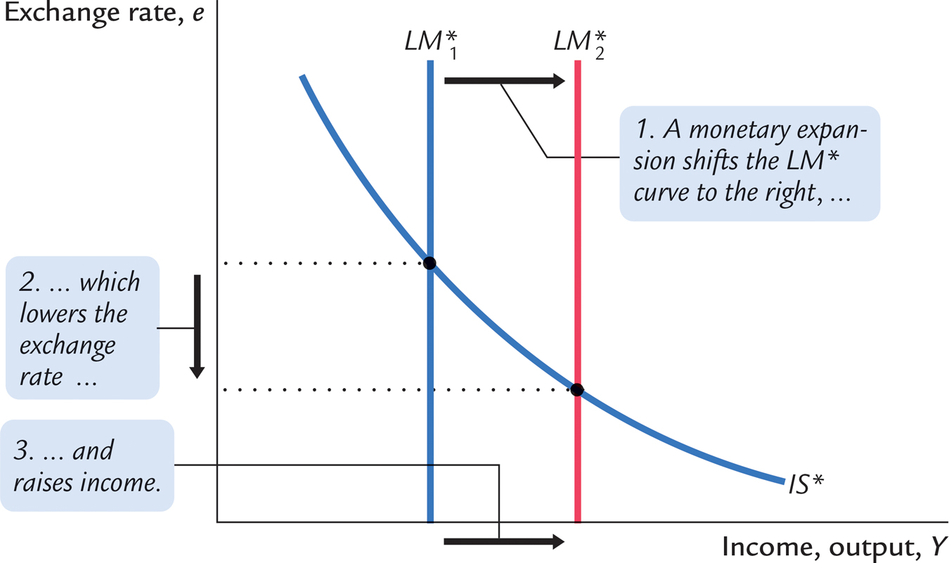
Suppose now that the central bank increases the money supply. Because the price level is assumed to be fixed, the increase in the money supply means an increase in real money balances. The increase in real balances shifts the LM* curve to the right, as in Figure 13-5. Hence, an increase in the money supply raises income and lowers the exchange rate.

376

Although monetary policy influences income in an open economy, as it does in a closed economy, the monetary transmission mechanism is different. Recall that in a closed economy an increase in the money supply increases spending because it lowers the interest rate and stimulates investment. In a small open economy, this channel of monetary transmission is not available because the interest rate is fixed by the world interest rate. So how does monetary policy influence spending? To answer this question, we once again need to think about the international flow of capital and its implications for the domestic economy.

The interest rate and the exchange rate are again the key variables. As soon as an increase in the money supply starts putting downward pressure on the domestic interest rate, capital flows out of the economy because investors seek a higher return elsewhere. This capital outflow prevents the domestic interest rate from falling below the world interest rate r*. It also has another effect: because investing abroad requires converting domestic currency into foreign currency, the capital outflow increases the supply of the domestic currency in the market for foreign-currency exchange, causing the domestic currency to depreciate in value. This depreciation makes domestic goods less expensive relative to foreign goods, stimulating net exports and thus total income. Hence, in a small open economy, monetary policy influences income by altering the exchange rate rather than the interest rate.

Suppose that the government reduces the demand for imported goods by imposing an import quota or a tariff. What happens to aggregate income and the exchange rate? How does the economy reach its new equilibrium?

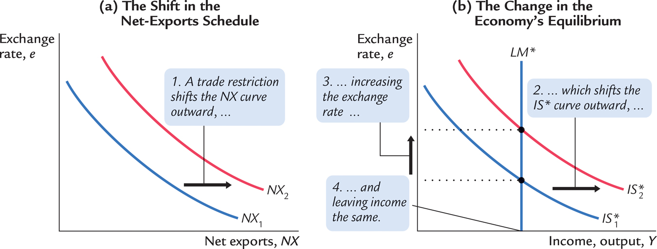
Because net exports equal exports minus imports, a reduction in imports means an increase in net exports. That is, the net-exports schedule shifts to the right, as in Figure 13-6. This shift in the net-exports schedule increases planned expenditure and thus moves the IS* curve to the right. Because the LM* curve is vertical, the trade restriction raises the exchange rate but does not affect income.

The economic forces behind this transition are similar to the case of expansionary fiscal policy. Because net exports are a component of GDP, the rightward shift in the net-exports schedule, other things equal, puts upward pressure on income Y; an increase in Y, in turn, increases money demand and puts upward pressure on the interest rate r. Foreign capital quickly responds by flowing into the domestic economy, pushing the interest rate back to the world interest rate r* and causing the domestic currency to appreciate in value. Finally, the appreciation of the currency makes domestic goods more expensive relative to foreign goods, which decreases net exports NX and returns income Y to its initial level.

Restrictive trade policies often have the goal of changing the trade balance NX. Yet, as we first saw in Chapter 6, such policies do not necessarily have that effect. The same conclusion holds in the Mundell–Fleming model under floating exchange rates. Recall that

NX(e) = Y − C(Y − T) − I(r*) − G.

377

Because a trade restriction does not affect income, consumption, investment, or government purchases, it does not affect the trade balance. Although the shift in the net-exports schedule tends to raise NX, the increase in the exchange rate reduces NX by the same amount. The overall effect is simply less trade. The domestic economy imports less than it did before the trade restriction, but it exports less as well.