PROBLEMS AND APPLICATIONS
To access online learning resources, visit  for Macroeconomics, 9e at www.macmillanhighered.com/launchpad/mankiw9e
Question 16.7
1. The chapter uses the Fisher model to discuss a change in the interest rate for a consumer who saves some of his first-period income. Suppose, instead, that the consumer is a borrower. How does that alter the analysis? Discuss the income and substitution effects on consumption in both periods.
Question 16.8
2. Gabe and Gita both obey the two-period Fisher model of consumption. Gabe earns $100 in the first period and $100 in the second period. Gita earns nothing in the first period and $210 in the second period. Both of them can borrow or lend at the interest rate r.
You observe both Gabe and Gita consuming $100 in the first period and $100 in the second period. What is the interest rate r?
Suppose the interest rate increases. What will happen to Gabe’s consumption in the first period? Is Gabe better off or worse off than before the interest rate rise?
What will happen to Gita’s consumption in the first period when the interest rate increases? Is Gita better off or worse off than before the interest rate increase?
Question 16.9
3. The chapter analyzes Fisher’s model for the case in which the consumer can save or borrow at an interest rate of r and for the case in which the consumer can save at this rate but cannot borrow at all. Consider now the intermediate case in which the consumer can save at rate rs and borrow at rate rb, where rs < rb.
What is the consumer’s budget constraint in the case in which he consumes less than his income in period one? Answer in the form of an equation.
What is the consumer’s budget constraint in the case in which he consumes more than his income in period one? Answer in the form of an equation.
On a single graph, show the two budget constraints from parts (a) and (b). Shade the area that represents the combination of first-period and second-period consumption the consumer can choose.
Now add to your graph the consumer’s indifference curves. Show three possible outcomes: one in which the consumer saves, one in which he borrows, and one in which he neither saves nor borrows.
What determines first-period consumption in each of the three cases?
Question 16.10
4. Explain whether borrowing constraints increase or decrease the potency of fiscal policy to influence aggregate demand in each of the following cases.
A temporary tax cut
An announced future tax cut
505
Question 16.11
5. Albert and Franco both follow the life-cycle hypothesis: they smooth consumption as much as possible. They each live for five periods, the last two of which are retirement. Here are their incomes earned during each period:
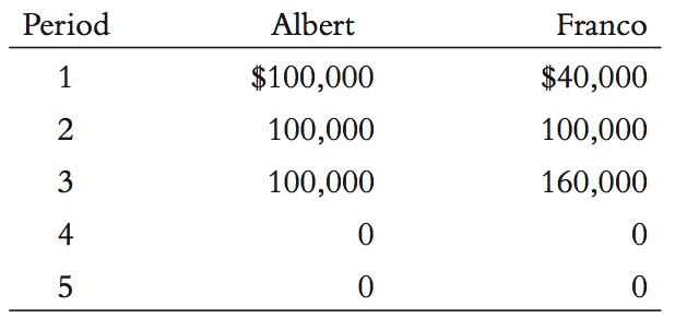
They both die at the beginning of period six. To keep things simple, assume that the interest rate is zero for both saving and borrowing and that the life span is perfectly predictable.
For each individual, compute consumption and saving in each period of life.
Compute their wealth (that is, their accumulated saving) at the beginning of each period, including period six.
Graph consumption, income, and wealth for each of them, with the period on the horizontal axis. Compare your graph to Figure 16-12.
Suppose now that consumers cannot borrow, so wealth cannot be negative. How does that change your answers above? Draw a new graph for part (c) if necessary.
Question 16.12
6. Demographers predict that the fraction of the population that is elderly will increase over the next 20 years. What does the life-cycle model predict for the influence of this demographic change on the national saving rate?
Question 16.13
7. A Case Study in the chapter indicates that the elderly do not dissave as much as the life-cycle model predicts.
Describe the two possible explanations for this phenomenon.
One study found that the elderly who do not have children dissave at about the same rate as the elderly who do have children. What might this finding imply about the validity of the two explanations? Why might it be inconclusive?
Question 16.14
8. Consider two savings accounts that pay the same interest rate. One account lets you take your money out on demand. The second requires that you give 30-day advance notification before withdrawals.
Which account would you prefer? Why?
Can you imagine a person who might make the opposite choice? Explain.
What do these choices say about the theories of the consumption function discussed in this chapter?
Question 16.15
9. This problem uses calculus to compare two scenarios of consumer optimization.
Nina has the following utility function:
U = ln(C1) + ln(C2) + ln(C3).
She starts with wealth of $120,000, earns no additional income, and faces a zero interest rate. How much does she consume in each of the three periods? (Hint: The marginal rate of substitution between consumption in any two periods is the ratio of marginal utilities.)
David is just like Nina, except he always gets extra utility from present consumption. From the perspective of period one, his utility function is
U = 2 ln(C1) + ln(C2) + ln(C3).
In period one, how much does David decide to consume in each of the three periods? How much wealth does he have left after period one?
When David enters period two, his utility function is
U = ln(C1) + 2 ln(C2) + ln(C3).
How much does he consume in periods two and three? How does your answer here compare to David’s decision in part (b)?
If, in period one, David were able to constrain the choices he can make in period two, what would he do? Relate this example to one of the theories of consumption discussed in the chapter.
1 For references to the large body of work on the life-cycle hypothesis, a good place to start is the lecture Modigliani gave when he won the Nobel Prize: Franco Modigliani, “Life Cycle, Individual Thrift, and the Wealth of Nations,” American Economic Review 76 (June 1986): 297–313. For an example of more recent research in this tradition, see Pierre-Olivier Gourinchas and Jonathan A. Parker, “Consumption Over the Life Cycle,” Econometrica 70 (January 2002): 47–89.
2 To read more about the consumption and saving of the elderly, see Albert Ando and Arthur Kennickell, “How Much (or Little) Life Cycle Saving Is There in Micro Data?” in Rudiger Dornbusch, Stanley Fischer, and John Bossons, eds., Macroeconomics and Finance: Essays in Honor of Franco Modigliani (Cambridge, MA: MIT Press, 1986): 159–223; and Michael Hurd, “Research on the Elderly: Economic Status, Retirement, and Consumption and Saving,” Journal of Economic Literature 28 (June 1990): 565–589.
3 Milton Friedman, A Theory of the Consumption Function (Princeton, NJ: Princeton University Press, 1957).
4 Jonathan A. Parker, Nicholas S. Souleles, David S. Johnson, and Robert McClelland,“Consumer Spending and the Economic Stimulus Payments of 2008,” American Economic Review 103 (October 2013): 2530–2553.
5 Robert E. Hall, “Stochastic Implications of the Life Cycle–Permanent Income Hypothesis: Theory and Evidence,” Journal of Political Economy 86 (December 1978): 971–987.
6 John Y. Campbell and N. Gregory Mankiw, “Consumption, Income, and Interest Rates: Reinterpreting the Time-Series Evidence,” NBER Macroeconomics Annual (1989): 185–216; Jonathan Parker, “The Response of Household Consumption to Predictable Changes in Social Security Taxes,” American Economic Review 89 (September 1999): 959–973; Nicholas S. Souleles, “The Response of Household Consumption to Income Tax Refunds,” American Economic Review 89 (September 1999): 947–958.
7 For more on this topic, see David Laibson, “Golden Eggs and Hyperbolic Discounting,” Quarterly Journal of Economics 62 (May 1997): 443–477; and George-Marios Angeletos, David Laibson, Andrea Repetto, Jeremy Tobacman, and Stephen Weinberg, “The Hyperbolic Buffer Stock Model: Calibration, Simulation, and Empirical Evidence,” Journal of Economic Perspectives 15 (Summer 2001): 47–68.
8 James J. Choi, David I. Laibson, Brigitte Madrian, and Andrew Metrick, “Defined Contribution Pensions: Plan Rules, Participant Decisions, and the Path of Least Resistance,” Tax Policy and the Economy 16 (2002): 67–113; Richard H. Thaler and Shlomo Benartzi, “Save More Tomorrow: Using Behavioral Economics to Increase Employee Saving,” Journal of Political Economy 112 (2004): S164–S187.
506