The consumption function introduced by Keynes relates current consumption to current income. This relationship, however, is incomplete at best. When people decide how much to consume and how much to save, they consider both the present and the future. The more consumption they enjoy today, the less they will be able to enjoy tomorrow. In making this tradeoff, households must look ahead to the income they expect to receive in the future and to the consumption of goods and services they hope to be able to afford.

The economist Irving Fisher developed the model with which economists analyze how rational, forward-looking consumers make intertemporal choices—that is, choices involving different periods of time. Fisher’s model illuminates the constraints consumers face, the preferences they have, and how these constraints and preferences together determine their choices about consumption and saving.

Most people would prefer to increase the quantity or quality of the goods and services they consume—to wear nicer clothes, eat at better restaurants, or see more movies. The reason people consume less than they desire is that their consumption is constrained by their income. In other words, consumers face a limit on how much they can spend, called a budget constraint. When they are deciding how much to consume today versus how much to save for the future, they face an intertemporal budget constraint, which measures the total resources available for consumption today and in the future. Our first step in developing Fisher’s model is to examine this constraint in some detail.

To keep things simple, we examine the decision facing a consumer who lives for two periods. Period one represents the consumer’s youth, and period two represents the consumer’s old age. The consumer earns income Y₁ and consumes C₁ in period one, and earns income Y₂ and consumes C₂ in period two. (All variables are real—that is, adjusted for inflation.) Because the consumer has the opportunity to borrow and save, consumption in any single period can be either greater or less than income in that period.

Consider how the consumer’s income in the two periods constrains consumption in the two periods. In the first period, saving equals income minus consumption. That is,

S = Y₁ − C₁,

where S is saving. In the second period, consumption equals the accumulated saving, including the interest earned on that saving, plus second-period income. That is,

C₂ = (1 + r)S + Y₂,

where r is the real interest rate. For example, if the real interest rate is 5 percent, then for every $1 of saving in period one, the consumer enjoys an extra $1.05 of consumption in period two. Because there is no third period, the consumer does not save in the second period.

481

Note that the variable S can represent either saving or borrowing and that these equations hold in both cases. If first-period consumption is less than first-period income, the consumer is saving, and S is greater than zero. If first-period consumption exceeds first-period income, the consumer is borrowing, and S is less than zero. For simplicity, we assume that the interest rate for borrowing is the same as the interest rate for saving.

To derive the consumer’s budget constraint, combine the two preceding equations. Substitute the first equation for S into the second equation to obtain

C₂ = (1 + r)(Y₁ − C₁) + Y₂.

To make the equation easier to interpret, we must rearrange terms. To place all the consumption terms together, bring (1 + r)C₁ from the right-hand side to the left-hand side of the equation to obtain

(1 + r)C₁ + C₂ = (1 + r)Y₁ + Y₂.

Now divide both sides by 1 + r to obtain

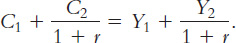
This equation relates consumption in the two periods to income in the two periods. It is the standard way of expressing the consumer’s intertemporal budget constraint.

The consumer’s budget constraint is easily interpreted. If the interest rate is zero, the budget constraint shows that total consumption in the two periods equals total income in the two periods. In the usual case in which the interest rate is greater than zero, future consumption and future income are discounted by a factor 1 + r. This discounting arises from the interest earned on savings. In essence, because the consumer earns interest on current income that is saved, future income is worth less than current income. Similarly, because future consumption is paid for out of savings that have earned interest, future consumption costs less than current consumption. The factor 1/(1 + r) is the price of second-period consumption measured in terms of first-period consumption: it is the amount of first-period consumption that the consumer must forgo to obtain 1 unit of second-period consumption.

Figure 16-3 graphs the consumer’s budget constraint. Three points are marked on this figure. At point A, the consumer consumes exactly his income in each period (C₁ = Y₁ and C₂ = Y₂), so there is neither saving nor borrowing between the two periods. At point B, the consumer consumes nothing in the first period (C₁ = 0) and saves all income, so second-period consumption C₂ is (1 + r)Y₁ + Y₂. At point C, the consumer plans to consume nothing in the second period (C₂ = 0) and borrows as much as possible against second-period income, so first-period consumption C₁ is Y₁ + Y₂/(1 + r). These are only three of the many combinations of first- and second-period consumption that the consumer can afford: all the points on the line from B to C are available to the consumer.

482

483

The consumer’s preferences regarding consumption in the two periods can be represented by indifference curves. An indifference curve shows the combinations of first-period and second-period consumption that make the consumer equally happy.

Figure 16-4 shows two of the consumer’s many indifference curves. The consumer is indifferent among combinations W, X, and Y because they are all on the same curve. Not surprisingly, if the consumer’s first-period consumption is reduced—say, from point W to point X—second-period consumption must increase to keep him equally happy. If first-period consumption is reduced again, from point X to point Y, the amount of extra second-period consumption he requires for compensation is greater.

The slope at any point on the indifference curve shows how much second-period consumption the consumer requires in order to be compensated for a 1-unit reduction in first-period consumption. This slope is the marginal rate of substitution between first-period consumption and second-period consumption. It tells us the rate at which the consumer is willing to substitute second-period consumption for first-period consumption.

Notice that the indifference curves in Figure 16-4 are not straight lines; as a result, the marginal rate of substitution depends on the levels of consumption in the two periods. When first-period consumption is high and second-period consumption is low, as at point W, the marginal rate of substitution is low: the consumer requires only a little extra second-period consumption to give up 1 unit of first-period consumption. When first-period consumption is low and second-period consumption is high, as at point Y, the marginal rate of substitution is high: the consumer requires much additional second-period consumption to give up 1 unit of first-period consumption.

484

The consumer is equally happy at all points on a given indifference curve, but he prefers some indifference curves to others. Because he prefers more consumption to less, he prefers higher indifference curves to lower ones. In Figure 16-4, the consumer prefers any of the points on curve IC₂ to any of the points on curve IC₁.

The set of indifference curves gives a complete ranking of the consumer’s preferences. It tells us that the consumer prefers point Z to point W, but that should be obvious because point Z has more consumption in both periods. Yet compare point Z and point Y: point Z has more consumption in period one and less in period two. Which is preferred, Z or Y? Because Z is on a higher indifference curve than Y, we know that the consumer prefers point Z to point Y. Hence, we can use the set of indifference curves to rank any combinations of first-period and second-period consumption.

Having discussed the consumer’s budget constraint and preferences, we can consider the decision about how much to consume in each period of time. The consumer would like to end up with the best possible combination of consumption in the two periods—that is, on the highest possible indifference curve. But the budget constraint requires that the consumer also end up on or below the budget line because the budget line measures the total resources available to him.

Figure 16-5 shows that many indifference curves cross the budget line. The highest indifference curve that the consumer can obtain without violating the budget constraint is the indifference curve that just barely touches the budget line, which is curve IC₃ in the figure. The point at which the curve and line touch—point O, for “optimum”—is the best combination of consumption in the two periods that the consumer can afford.

485

Notice that, at the optimum, the slope of the indifference curve equals the slope of the budget line. The indifference curve is tangent to the budget line. The slope of the indifference curve is the marginal rate of substitution MRS, and the slope of the budget line is 1 plus the real interest rate. We conclude that at point O

MRS = 1 + r.

The consumer chooses consumption in the two periods such that the marginal rate of substitution equals 1 plus the real interest rate.

Now that we have seen how the consumer makes the consumption decision, let’s examine how consumption responds to an increase in income. An increase in either Y₁ or Y₂ shifts the budget constraint outward, as in Figure 16-6. The higher budget constraint allows the consumer to choose a better combination of first- and second-period consumption—that is, the consumer can now reach a higher indifference curve.

In Figure 16-6, the consumer responds to the shift in his budget constraint by choosing more consumption in both periods. Although it is not implied by the logic of the model alone, this situation is the most usual. If a consumer wants more of a good when his income rises, economists call it a normal good. The indifference curves in Figure 16-6 are drawn under the assumption that consumption in period one and consumption in period two are both normal goods.

486

The key conclusion from Figure 16-6 is that regardless of whether the increase in income occurs in the first period or the second period, the consumer spreads it over consumption in both periods. This behavior is sometimes called consumption smoothing. Because the consumer can borrow and lend between periods, the timing of the income is irrelevant to how much is consumed today (except that future income is discounted by the interest rate). The lesson of this analysis is that consumption depends on the present value of current and future income, which can be written as

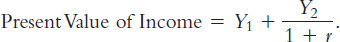
Notice that this conclusion is quite different from that reached by Keynes. Keynes posited that a person’s current consumption depends largely on his current income. Fisher’s model says, instead, that consumption is based on the income the consumer expects over his entire lifetime.

Let’s now use Fisher’s model to consider how a change in the real interest rate alters the consumer’s choices. There are two cases to consider: the case in which the consumer is initially saving and the case in which he is initially borrowing. Here we discuss the saving case; Problem 1 at the end of the chapter asks you to analyze the borrowing case.

Figure 16-7 shows that an increase in the real interest rate rotates the consumer’s budget line around the point (Y₁, Y₂) and, thereby, alters the amount of consumption he chooses in both periods. Here, the consumer moves from point A to point B. You can see that for the indifference curves drawn in this figure, first-period consumption falls and second-period consumption rises.

Economists decompose the impact of an increase in the real interest rate on consumption into two effects: an income effect and a substitution effect. Textbooks on microeconomics discuss these effects in detail. We summarize them briefly here.

The income effect is the change in consumption that results from the movement to a higher indifference curve. Because the consumer is a saver rather than a borrower (as indicated by the fact that first-period consumption is less than first-period income), the increase in the interest rate makes him better off (as reflected by the movement to a higher indifference curve). If consumption in period one and consumption in period two are both normal goods, the consumer will want to spread this improvement in his welfare over both periods. This income effect tends to make the consumer want more consumption in both periods.

The substitution effect is the change in consumption that results from the change in the relative price of consumption in the two periods. In particular, consumption in period two becomes less expensive relative to consumption in period one when the interest rate rises. That is, because the real interest rate earned on saving is higher, the consumer must now give up less first-period consumption to obtain an extra unit of second-period consumption. This substitution effect tends to make the consumer choose more consumption in period two and less consumption in period one.

487

The consumer’s choice depends on both the income effect and the substitution effect. Because both effects act to increase the amount of second-period consumption, we can conclude that an increase in the real interest rate raises second-period consumption. But the two effects have opposite impacts on first-period consumption, so the increase in the interest rate could either lower or raise it. Hence, depending on the relative size of income and substitution effects, an increase in the interest rate could either stimulate or depress saving.

Fisher’s model assumes that the consumer can borrow as well as save. The ability to borrow allows current consumption to exceed current income. In essence, when the consumer borrows, he consumes some of his future income today. Yet for many people such borrowing is impossible. For example, a student wishing to enjoy spring break in Florida would probably be unable to finance this vacation with a bank loan. Let’s examine how Fisher’s analysis changes if the consumer cannot borrow.

488

The inability to borrow prevents current consumption from exceeding current income. A constraint on borrowing can therefore be expressed as

C₁ ≤ Y₁.

This inequality states that consumption in period one must be less than or equal to income in period one. This additional constraint on the consumer is called a borrowing constraint or, sometimes, a liquidity constraint.

Figure 16-8 shows how this borrowing constraint restricts the consumer’s set of choices. The consumer’s choice must satisfy both the intertemporal budget constraint and the borrowing constraint. The shaded area represents the combinations of first-period consumption and second-period consumption that satisfy both constraints.

Figure 16-9 shows how this borrowing constraint affects the consumption decision. There are two possibilities. In panel (a), the consumer wishes to consume less in period one than he earns. The borrowing constraint is not binding and, therefore, does not affect consumption. In panel (b), the consumer would like to choose point D, where he consumes more in period one than he earns, but the borrowing constraint prevents this outcome. The best the consumer can do is to consume all of his first-period income, represented by point E.

The analysis of borrowing constraints leads us to conclude that there are two consumption functions. For some consumers, the borrowing constraint is not binding, and consumption in both periods depends on the present value of lifetime income, Y₁ + [Y₂/(1 + r)]. For other consumers, the borrowing constraint binds, and the consumption function is C₁ = Y₁ and C₂ = Y₂. Hence, for those consumers who would like to borrow but cannot, consumption depends only on current income.

489