5-1 The Quantity Theory of Money
In Chapter 4 we defined what money is and learned that the quantity of money available in the economy is called the money supply. We also saw how the money supply is determined by the banking system together with the policy decisions of the central bank. With that foundation, we can now start to examine the broad macroeconomic effects of monetary policy. To do this, we need a theory that tells us how the quantity of money is related to other economic variables, such as prices and incomes. The theory we develop in this section, called the quantity theory of money, has its roots in the work of the early monetary theorists, including the philosopher and economist David Hume (1711–
Transactions and the Quantity Equation
If you hear an economist use the word “supply,” you can be sure that the word “demand” is not far behind. Indeed, having fully explored the supply of money, we now focus on the demand for it.
107
The starting point of the quantity theory of money is the insight that people hold money to buy goods and services. The more money they need for such transactions, the more money they hold. Thus, the quantity of money in the economy is related to the number of dollars exchanged in transactions.
The link between transactions and money is expressed in the following equation, called the quantity equation:
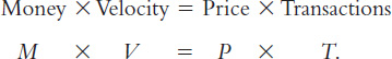
Let’s examine each of the four variables in this equation.
The right-
The left-
For example, suppose that 60 loaves of bread are sold in a given year at $0.50 per loaf. Then T equals 60 loaves per year, and P equals $0.50 per loaf. The total number of dollars exchanged is
PT = $0.50/loaf × 60 loaves/year = $30/year.
The right-
Suppose further that the quantity of money in the economy is $10. By rearranging the quantity equation, we can compute velocity as
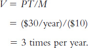
That is, for $30 of transactions per year to take place with $10 of money, each dollar must change hands three times per year.
The quantity equation is an identity: the definitions of the four variables make it true. This type of equation is useful because it shows that if one of the variables changes, one or more of the others must also change to maintain the equality. For example, if the quantity of money increases and the velocity of money remains unchanged, then either the price or the number of transactions must rise.
108
From Transactions to Income
When studying the role of money in the economy, economists usually use a slightly different version of the quantity equation than the one just introduced. The problem with the first equation is that the number of transactions is difficult to measure. To solve this problem, the number of transactions T is replaced by the total output of the economy Y.
Transactions and output are related because the more the economy produces, the more goods are bought and sold. They are not the same, however. When one person sells a used car to another person, for example, they make a transaction using money, even though the used car is not part of current output. Nonetheless, the dollar value of transactions is roughly proportional to the dollar value of output.
If Y denotes the amount of output and P denotes the price of one unit of output, then the dollar value of output is PY. We encountered measures for these variables when we discussed the national income accounts in Chapter 2: Y is real GDP; P, the GDP deflator; and PY, nominal GDP. The quantity equation becomes

Because Y is also total income, V in this version of the quantity equation is called the income velocity of money. The income velocity of money tells us the number of times a dollar bill enters someone’s income in a given period of time. This version of the quantity equation is the most common, and it is the one we use from now on.
The Money Demand Function and the Quantity Equation
When we analyze how money affects the economy, it is often useful to express the quantity of money in terms of the quantity of goods and services it can buy. This amount, M/P, is called real money balances.
Real money balances measure the purchasing power of the stock of money. For example, consider an economy that produces only bread. If the quantity of money is $10, and the price of a loaf is $0.50, then real money balances are 20 loaves of bread. That is, at current prices, the stock of money in the economy is able to buy 20 loaves.
A money demand function is an equation that shows the determinants of the quantity of real money balances people wish to hold. A simple money demand function is
(M/P)d = kY,
where k is a constant that tells us how much money people want to hold for every dollar of income. This equation states that the quantity of real money balances demanded is proportional to real income.
109
The money demand function is like the demand function for a particular good. Here the “good” is the convenience of holding real money balances. Just as owning an automobile makes it easier for a person to travel, holding money makes it easier to make transactions. Therefore, just as higher income leads to a greater demand for automobiles, higher income also leads to a greater demand for real money balances.
This money demand function offers another way to view the quantity equation. To see this, add to the money demand function the condition that the demand for real money balances (M/P)d must equal the supply M/P. Therefore,
M/P = kY.
A simple rearrangement of terms changes this equation into
M(1/k) = PY,
which can be written as
MV = PY,
where V = 1/k. These few steps of simple mathematics show the link between the demand for money and the velocity of money. When people want to hold a lot of money for each dollar of income (k is large), money changes hands infrequently (V is small). Conversely, when people want to hold only a little money (k is small), money changes hands frequently (V is large). In other words, the money demand parameter k and the velocity of money V are opposite sides of the same coin.
The Assumption of Constant Velocity
The quantity equation can be viewed as a definition: it defines velocity V as the ratio of nominal GDP, PY, to the quantity of money M. Yet if we make the additional assumption that the velocity of money is constant, then the quantity equation becomes a useful theory about the effects of money, called the quantity theory of money.
Like many of the assumptions in economics, the assumption of constant velocity is only a simplification of reality. Velocity does change if the money demand function changes. For example, when automatic teller machines were introduced, people could reduce their average money holdings, which meant a fall in the money demand parameter k and an increase in velocity V. Nonetheless, experience shows that the assumption of constant velocity is a useful one in many situations. Let’s therefore assume that velocity is constant and see what this assumption implies about the effects of the money supply on the economy.
With this assumption included, the quantity equation can be seen as a theory of what determines nominal GDP. The quantity equation says

where the bar over V means that velocity is fixed. Therefore, a change in the quantity of money (M) must cause a proportionate change in nominal GDP (PY). That is, if velocity is fixed, the quantity of money determines the dollar value of the economy’s output.
110
Money, Prices, and Inflation
We now have a theory to explain what determines the economy’s overall level of prices. The theory has three building blocks:
The factors of production and the production function determine the level of output Y. We borrow this conclusion from Chapter 3.
The money supply M set by the central bank determines the nominal value of output PY. This conclusion follows from the quantity equation and the assumption that the velocity of money is fixed.
The price level P is then the ratio of the nominal value of output PY to the level of output Y.
In other words, the productive capability of the economy determines real GDP, the quantity of money determines nominal GDP, and the GDP deflator is the ratio of nominal GDP to real GDP.
This theory explains what happens when the central bank changes the supply of money. Because velocity V is fixed, any change in the money supply M must lead to a proportionate change in the nominal value of output PY. Because the factors of production and the production function have already determined output Y, the nominal value of output PY can adjust only if the price level P changes. Hence, the quantity theory implies that the price level is proportional to the money supply.
Because the inflation rate is the percentage change in the price level, this theory of the price level is also a theory of the inflation rate. The quantity equation, written in percentage-
% Change in M + % Change in V = % Change in P + % Change in Y.
Consider each of these four terms. First, the percentage change in the quantity of money M is under the control of the central bank. Second, the percentage change in velocity V reflects shifts in money demand; we have assumed that velocity is constant, so the percentage change in velocity is zero. Third, the percentage change in the price level P is the rate of inflation; this is the variable in the equation that we would like to explain. Fourth, the percentage change in output Y depends on growth in the factors of production and on technological progress, which for our present purposes we are taking as given. This analysis tells us that (except for a constant that depends on exogenous growth in output) the growth in the money supply determines the rate of inflation.
Thus, the quantity theory of money states that the central bank, which controls the money supply, has ultimate control over the rate of inflation. If the central bank keeps the money supply stable, the price level will be stable. If the central bank increases the money supply rapidly, the price level will rise rapidly.
111
CASE STUDY
Inflation and Money Growth
“Inflation is always and everywhere a monetary phenomenon.” So wrote Milton Friedman, the great economist who won the Nobel Prize in economics in 1976. The quantity theory of money leads us to agree that the growth in the quantity of money is the primary determinant of the inflation rate. Yet Friedman’s claim is empirical, not theoretical. To evaluate his claim, and to judge the usefulness of our theory, we need to look at data on money and prices.
Friedman, together with fellow economist Anna Schwartz, wrote two treatises on monetary history that documented the sources and effects of changes in the quantity of money over the past century.1 Figure 5-1 uses some of their data and plots the average rate of money growth and the average rate of inflation in the United States over each decade since the 1870s. The data verify the link between inflation and growth in the quantity of money. Decades with high money growth (such as the 1970s) tend to have high inflation, and decades with low money growth (such as the 1930s) tend to have low inflation.
FIGURE 5-1

112
As you may have learned in a statistics class, one way to quantify a relationship between two variables is with a measure called correlation. A correlation is +1 if the two variables move exactly in tandem, 0 if they are unrelated, and −1 if they move exactly opposite each other. In Figure 5-1, the correlation is 0.79.
Figure 5-2 examines the same question using international data. It shows the average rate of inflation and the average rate of money growth in 126 countries during the period from 2000 to 2013. Again, the link between money growth and inflation is clear. Countries with high money growth (such as Angola and Belarus) tend to have high inflation, and countries with low money growth (such as Singapore and Switzerland) tend to have low inflation. The correlation here is 0.72.
FIGURE 5-2

If we looked at monthly data on money growth and inflation, rather than data for decade-
113