Having examined the international flows of capital and of goods and services, we now extend the analysis by considering the prices that apply to these transactions. The exchange rate between two countries is the price at which residents of those countries trade with each other. In this section we first examine precisely what the exchange rate measures and then discuss how exchange rates are determined.

Economists distinguish between two exchange rates: the nominal exchange rate and the real exchange rate. Let’s discuss each in turn and see how they are related.

The Nominal Exchange Rate The nominal exchange rate is the relative price of the currencies of two countries. For example, if the exchange rate between the U.S. dollar and the Japanese yen is 80 yen per dollar, then you can exchange one dollar for 80 yen in world markets for foreign currency. A Japanese who wants to obtain dollars would pay 80 yen for each dollar he bought. An American who wants to obtain yen would get 80 yen for each dollar he paid. When people refer to “the exchange rate” between two countries, they usually mean the nominal exchange rate.

156

Notice that an exchange rate can be reported in two ways. If one dollar buys 80 yen, then one yen buys 0.0125 dollar. We can say the exchange rate is 80 yen per dollar, or we can say the exchange rate is 0.0125 dollar per yen. Because 0.0125 equals 1/80, these two ways of expressing the exchange rate are equivalent.

This book always expresses the exchange rate in units of foreign currency per dollar. With this convention, a rise in the exchange rate—say, from 80 to 100 yen per dollar—is called an appreciation of the dollar; a fall in the exchange rate is called a depreciation. When the domestic currency appreciates, it buys more of the foreign currency; when it depreciates, it buys less. An appreciation is sometimes called a strengthening of the currency, and a depreciation is sometimes called a weakening of the currency.

The Real Exchange Rate The real exchange rate is the relative price of the goods of two countries. That is, the real exchange rate tells us the rate at which we can trade the goods of one country for the goods of another. The real exchange rate is sometimes called the terms of trade.

To see the relation between the real and nominal exchange rates, consider a single good produced in many countries: cars. Suppose an American car costs $25,000 and a similar Japanese car costs 4,000,000 yen. To compare the prices of the two cars, we must convert them into a common currency. If a dollar is worth 80 yen, then the American car costs 80 × 25,000, or 2,000,000 yen. Comparing the price of the American car (2,000,000 yen) and the price of the Japanese car (4,000,000 yen), we conclude that the American car costs one-half of what the Japanese car costs. In other words, at current prices, we can exchange two American cars for one Japanese car.

We can summarize our calculation as follows:

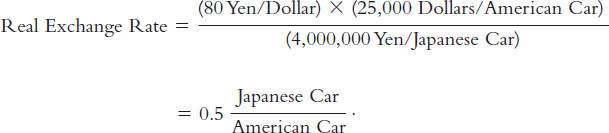
At these prices and this exchange rate, we obtain one-half of a Japanese car per American car. More generally, we can write this calculation as

The rate at which we exchange foreign and domestic goods depends on the prices of the goods in the local currencies and on the rate at which the currencies are exchanged.

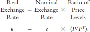
This calculation of the real exchange rate for a single good suggests how we should define the real exchange rate for a broader basket of goods. Let e be the nominal exchange rate (the number of yen per dollar), P be the price level in the United States (measured in dollars), and P* be the price level in Japan (measured in yen). Then the real exchange rate ε is

157

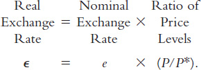
The real exchange rate between two countries is computed from the nominal exchange rate and the price levels in the two countries. If the real exchange rate is high, foreign goods are relatively cheap, and domestic goods are relatively expensive. If the real exchange rate is low, foreign goods are relatively expensive, and domestic goods are relatively cheap.

What macroeconomic influence does the real exchange rate exert? To answer this question, remember that the real exchange rate is nothing more than a relative price. Just as the relative price of hamburgers and pizza determines which you choose for lunch, the relative price of domestic and foreign goods affects the demand for these goods.

Suppose first that the real exchange rate is low. In this case, because domestic goods are relatively cheap, domestic residents will want to purchase fewer imported goods: they will buy Fords rather than Toyotas, drink Budweiser rather than Heineken, and vacation in Florida rather than Italy. For the same reason, foreigners will want to buy many of our goods. As a result of both of these actions, the quantity of our net exports demanded will be high.

The opposite occurs if the real exchange rate is high. Because domestic goods are expensive relative to foreign goods, domestic residents will want to buy many imported goods, and foreigners will want to buy few of our goods. Therefore, the quantity of our net exports demanded will be low.

We write this relationship between the real exchange rate and net exports as

NX = NX(ε).

This equation states that net exports are a function of the real exchange rate. Figure 6-7 illustrates the negative relationship between the trade balance and the real exchange rate.

We now have all the pieces needed to construct a model that explains what factors determine the real exchange rate. In particular, we combine the relationship between net exports and the real exchange rate we just discussed with the model of the trade balance we developed earlier in the chapter. We can summarize the analysis as follows:

158

Figure 6-8 illustrates these two conditions. The line showing the relationship between net exports and the real exchange rate slopes downward because a low real exchange rate makes domestic goods relatively inexpensive. The line representing the excess of saving over investment, S – I, is vertical because neither saving nor investment depends on the real exchange rate. The crossing of these two lines determines the equilibrium real exchange rate.

159

Figure 6-8 looks like an ordinary supply-and-demand diagram. In fact, you can think of this diagram as representing the supply and demand for foreign-currency exchange. The vertical line, S – I, represents the net capital outflow and thus the supply of dollars to be exchanged into foreign currency and invested abroad. The downward-sloping line, NX(ε), represents the net demand for dollars coming from foreigners who want dollars to buy our goods. At the equilibrium real exchange rate, the supply of dollars available from the net capital outflow balances the demand for dollars by foreigners buying our net exports.

We can use this model to show how the changes in economic policy we discussed earlier affect the real exchange rate.

Fiscal Policy at Home What happens to the real exchange rate if the government reduces national saving by increasing government purchases or cutting taxes? As we discussed earlier, this reduction in saving lowers S – I and thus NX. That is, the reduction in saving causes a trade deficit.

Figure 6-9 shows how the equilibrium real exchange rate adjusts to ensure that NX falls. The change in policy shifts the vertical S – I line to the left, lowering the supply of dollars to be invested abroad. The lower supply causes the equilibrium real exchange rate to rise from ε₁ to ε₂—that is, the dollar becomes more valuable. Because of the rise in the value of the dollar, domestic goods become more expensive relative to foreign goods, which causes exports to fall and imports to rise. The change in exports and the change in imports both act to reduce net exports.

160

Fiscal Policy Abroad What happens to the real exchange rate if foreign governments increase government purchases or cut taxes? Either change in fiscal policy reduces world saving and raises the world interest rate. The increase in the world interest rate reduces domestic investment I, which raises S – I and thus NX. That is, the increase in the world interest rate causes a trade surplus.

Figure 6-10 shows that this change in policy shifts the vertical S – I line to the right, raising the supply of dollars to be invested abroad. The equilibrium real exchange rate falls. That is, the dollar becomes less valuable, and domestic goods become less expensive relative to foreign goods.

Shifts in Investment Demand What happens to the real exchange rate if investment demand at home increases, perhaps because Congress passes an investment tax credit? At the given world interest rate, the increase in investment demand leads to higher investment. A higher value of I means lower values of S – I and NX. That is, the increase in investment demand causes a trade deficit.

Figure 6-11 shows that the increase in investment demand shifts the vertical S – I line to the left, reducing the supply of dollars to be invested abroad. The equilibrium real exchange rate rises. Hence, when the investment tax credit makes investing in the United States more attractive, it also increases the value of the U.S. dollars necessary to make these investments. When the dollar appreciates, domestic goods become more expensive relative to foreign goods, and net exports fall.

Now that we have a model that explains the trade balance and the real exchange rate, we have the tools to examine the macroeconomic effects of trade policies. Trade policies, broadly defined, are policies designed to directly influence the amount of goods and services exported or imported. Most often, trade policies take the form of protecting domestic industries from foreign competition— either by placing a tax on foreign imports (a tariff) or restricting the amount of goods and services that can be imported (a quota).

161

For an example of a protectionist trade policy, consider what would happen if the government prohibited the import of foreign cars. For any given real exchange rate, imports would now be lower, implying that net exports (exports minus imports) would be higher. Thus, the net-exports schedule would shift outward, as in Figure 6-12. To see the effects of the policy, we compare the old equilibrium and the new equilibrium. In the new equilibrium, the real exchange rate is higher, and net exports are unchanged. Despite the shift in the net-exports schedule, the equilibrium level of net exports remains the same, because the protectionist policy does not alter either saving or investment.

This analysis shows that protectionist trade policies do not affect the trade balance. This surprising conclusion is often overlooked in the popular debate over trade policies. Because a trade deficit reflects an excess of imports over exports, one might guess that reducing imports—such as by prohibiting the import of foreign cars—would reduce a trade deficit. Yet our model shows that protectionist policies lead only to an appreciation of the real exchange rate. The increase in the price of domestic goods relative to foreign goods tends to lower net exports by stimulating imports and depressing exports. Thus, the appreciation offsets the increase in net exports that is directly attributable to the trade restriction.

Although protectionist trade policies do not alter the trade balance, they do affect the amount of trade. As we have seen, because the real exchange rate appreciates, the goods and services we produce become more expensive relative to foreign goods and services. We therefore export less in the new equilibrium. Because net exports are unchanged, we must import less as well. (The appreciation of the exchange rate does stimulate imports to some extent, but this only partly offsets the decrease in imports due to the trade restriction.) Thus, protectionist policies reduce both the quantity of imports and the quantity of exports.

162

This fall in the total amount of trade is the reason economists usually oppose protectionist policies. International trade benefits all countries by allowing each country to specialize in what it produces best and by providing each country with a greater variety of goods and services. Protectionist policies diminish these gains from trade. Although these policies benefit certain groups within society—for example, a ban on imported cars helps domestic car producers—society on average is worse off when policies reduce the amount of international trade.

Having seen what determines the real exchange rate, we now turn our attention to the nominal exchange rate—the rate at which the currencies of two countries trade. Recall the relationship between the real and the nominal exchange rate:

We can write the nominal exchange rate as

e = ε × (P*/P).

163

This equation shows that the nominal exchange rate depends on the real exchange rate and the price levels in the two countries. Given the value of the real exchange rate, if the domestic price level P rises, then the nominal exchange rate e will fall: because a dollar is worth less, a dollar will buy fewer yen. However, if the Japanese price level P* rises, then the nominal exchange rate will increase: because the yen is worth less, a dollar will buy more yen.

It is instructive to consider changes in exchange rates over time. The exchange rate equation can be written

% Change in e = % Change in ε + % Change in P* – % Change in P.

The percentage change in ε is the change in the real exchange rate. The percentage change in P is the domestic inflation rate π, and the percentage change in P* is the foreign country’s inflation rate π*. Thus, the percentage change in the nominal exchange rate is

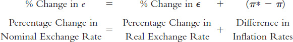
This equation states that the percentage change in the nominal exchange rate between the currencies of two countries equals the percentage change in the real exchange rate plus the difference in their inflation rates. If a country has a high rate of inflation relative to the United States, a dollar will buy an increasing amount of the foreign currency over time. If a country has a low rate of inflation relative to the United States, a dollar will buy a decreasing amount of the foreign currency over time.

This analysis shows how monetary policy affects the nominal exchange rate. We know from Chapter 5 that high growth in the money supply leads to high inflation. Here, we have just seen that one consequence of high inflation is a depreciating currency: high π implies falling e. In other words, just as growth in the amount of money raises the price of goods measured in terms of money, it also tends to raise the price of foreign currencies measured in terms of the domestic currency.

165

A famous hypothesis in economics, called the law of one price, states that the same good cannot sell for different prices in different locations at the same time. If a bushel of wheat sold for less in New York than in Chicago, it would be profitable to buy wheat in New York and then sell it in Chicago. This profit opportunity would become quickly apparent to astute arbitrageurs—people who specialize in “buying low” in one market and “selling high” in another. As the arbitrageurs took advantage of this opportunity, they would increase the demand for wheat in New York and increase the supply of wheat in Chicago. Their actions would drive the price up in New York and down in Chicago, thereby ensuring that prices are equalized in the two markets.

The law of one price applied to the international marketplace is called purchasing-power parity. It states that if international arbitrage is possible, then a dollar (or any other currency) must have the same purchasing power in every country. The argument goes as follows. If a dollar could buy more wheat domestically than abroad, there would be opportunities to profit by buying wheat domestically and selling it abroad. Profit-seeking arbitrageurs would drive up the domestic price of wheat relative to the foreign price. Similarly, if a dollar could buy more wheat abroad than domestically, the arbitrageurs would buy wheat abroad and sell it domestically, driving down the domestic price relative to the foreign price. Thus, profit-seeking by international arbitrageurs causes wheat prices to be the same in all countries.

We can interpret the doctrine of purchasing-power parity using our model of the real exchange rate. The quick action of these international arbitrageurs implies that net exports are highly sensitive to small movements in the real exchange rate. A small decrease in the price of domestic goods relative to foreign goods—that is, a small decrease in the real exchange rate—causes arbitrageurs to buy goods domestically and sell them abroad. Similarly, a small increase in the relative price of domestic goods causes arbitrageurs to import goods from abroad. Therefore, as in Figure 6-14, the net-exports schedule is very flat at the real exchange rate that equalizes purchasing power among countries: any small movement in the real exchange rate leads to a large change in net exports. This extreme sensitivity of net exports guarantees that the equilibrium real exchange rate is always close to the level that ensures purchasing-power parity.

166

Purchasing-power parity has two important implications. First, because the net-exports schedule is flat, changes in saving or investment do not influence the real or nominal exchange rate. Second, because the real exchange rate is fixed, all changes in the nominal exchange rate result from changes in price levels.

Is this doctrine of purchasing-power parity realistic? Most economists believe that, despite its appealing logic, purchasing-power parity does not provide a completely accurate description of the world. First, many goods are not easily traded. A haircut can be more expensive in Tokyo than in New York, yet there is no room for international arbitrage because it is impossible to transport haircuts. Second, even tradable goods are not always perfect substitutes. Some consumers prefer Toyotas, and others prefer Fords. Thus, the relative price of Toyotas and Fords can vary to some extent without leaving any profit opportunities. For these reasons, real exchange rates do in fact vary over time.

Although the doctrine of purchasing-power parity does not describe the world perfectly, it does provide a reason that movement in the real exchange rate will be limited. There is much validity to its underlying logic: the farther the real exchange rate drifts from the level predicted by purchasing-power parity, the greater the incentive for individuals to engage in international arbitrage in goods. We cannot rely on purchasing-power parity to eliminate all changes in the real exchange rate, but this doctrine does provide a reason to expect that fluctuations in the real exchange rate will typically be small or temporary.3