So far, we have used the Solow model to examine how an economy’s rate of saving and investment determines its steady-state levels of capital and income. This analysis might lead you to think that higher saving is always a good thing because it always leads to greater income. Yet suppose a nation had a saving rate of 100 percent. That would lead to the largest possible capital stock and the largest possible income. But if all of this income is saved and none is ever consumed, what good is it?

This section uses the Solow model to discuss the optimal amount of capital accumulation from the standpoint of economic well-being. In the next chapter, we discuss how government policies influence a nation’s saving rate. But first, in this section, we present the theory behind these policy decisions.

224

To keep our analysis simple, let’s assume that a policymaker can set the economy’s saving rate at any level. By setting the saving rate, the policymaker determines the economy’s steady state. What steady state should the policymaker choose?

The policymaker’s goal is to maximize the well-being of the individuals who make up the society. Individuals themselves do not care about the amount of capital in the economy or even the amount of output. They care about the amount of goods and services they can consume. Thus, a benevolent policymaker would want to choose the steady state with the highest level of consumption. The steady-state value of k that maximizes consumption is called the Golden Rule level of capital and is denoted .2

How can we tell whether an economy is at the Golden Rule level? To answer this question, we must first determine steady-state consumption per worker. Then we can see which steady state provides the most consumption.

To find steady-state consumption per worker, we begin with the national income accounts identity

y = c + i

and rearrange it as

c = y − i.

Consumption is output minus investment. Because we want to find steady-state consumption, we substitute steady-state values for output and investment. Steady-state output per worker is f(k*), where k* is the steady-state capital stock per worker. Furthermore, because the capital stock is not changing in the steady state, investment equals depreciation δk*. Substituting f(k*) for y and δk* for i, we can write steady-state consumption per worker as

c* = f(k*) − δk*.

According to this equation, steady-state consumption is what’s left of steady-state output after paying for steady-state depreciation. This equation shows that an increase in steady-state capital has two opposing effects on steady-state consumption. On the one hand, more capital means more output. On the other hand, more capital also means that more output must be used to replace capital that is wearing out.

Figure 8-7 graphs steady-state output and steady-state depreciation as a function of the steady-state capital stock. Steady-state consumption is the gap between output and depreciation. This figure shows that there is one level of the capital stock—the Golden Rule level —that maximizes consumption.

When comparing steady states, we must keep in mind that higher levels of capital affect both output and depreciation. If the capital stock is below the Golden Rule level, an increase in the capital stock raises output more than depreciation, so consumption rises. In this case, the production function is steeper than the δk* line, so the gap between these two curves—which equals consumption—grows as k* rises. By contrast, if the capital stock is above the Golden Rule level, an increase in the capital stock reduces consumption, because the increase in output is smaller than the increase in depreciation. In this case, the production function is flatter than the δk* line, so the gap between the curves—consumption—shrinks as k* rises. At the Golden Rule level of capital, the production function and the δk* line have the same slope, and consumption is at its greatest level.

225

We can now derive a simple condition that characterizes the Golden Rule level of capital. Recall that the slope of the production function is the marginal product of capital MPK. The slope of the δk* line is δ. Because these two slopes are equal at , the Golden Rule is described by the equation

MPK = δ.

At the Golden Rule level of capital, the marginal product of capital equals the depreciation rate.

To make the point somewhat differently, suppose that the economy starts at some steady-state capital stock k* and that the policymaker is considering increasing the capital stock to k* + 1. The amount of extra output from this increase in capital would be f(k* + 1) − f(k*), the marginal product of capital MPK. The amount of extra depreciation from having 1 more unit of capital is the depreciation rate δ. Thus, the net effect of this extra unit of capital on consumption is MPK − δ. If MPK − δ > 0, then increases in capital increase consumption, so k* must be below the Golden Rule level. If MPK − δ < 0, then increases in capital decrease consumption, so k* must be above the Golden Rule level. Therefore, the following condition describes the Golden Rule:

226

MPK − δ = 0.

At the Golden Rule level of capital, the marginal product of capital net of depreciation (MPK − δ) equals zero. As we will see, a policymaker can use this condition to find the Golden Rule capital stock for an economy.3

Keep in mind that the economy does not automatically gravitate toward the Golden Rule steady state. If we want any particular steady-state capital stock, such as the Golden Rule, we need a particular saving rate to support it. Figure 8-8 shows the steady state if the saving rate is set to produce the Golden Rule level of capital. If the saving rate is higher than the one used in this figure, the steady-state capital stock will be too high. If the saving rate is lower, the steady-state capital stock will be too low. In either case, steady-state consumption will be lower than it is at the Golden Rule steady state.

227

Consider the decision of a policymaker choosing a steady state in the following economy. The production function is the same as in our earlier example:

Output per worker is the square root of capital per worker. Depreciation δ is again 10 percent of capital. This time, the policymaker chooses the saving rate s and thus the economy’s steady state.

To see the outcomes available to the policymaker, recall that the following equation holds in the steady state:

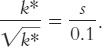
In this economy, this equation becomes

Squaring both sides of this equation yields a solution for the steady-state capital stock. We find

k* = 100s².

Using this result, we can compute the steady-state capital stock for any saving rate.

Table 8-3 presents calculations showing the steady states that result from various saving rates in this economy. We see that higher saving leads to a higher capital stock, which in turn leads to higher output and higher depreciation. Steady-state consumption, the difference between output and depreciation, first rises with higher saving rates and then declines. Consumption is highest when the saving rate is 0.5. Hence, a saving rate of 0.5 produces the Golden Rule steady state.

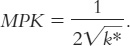
Recall that another way to identify the Golden Rule steady state is to find the capital stock at which the net marginal product of capital (MPK − δ) equals zero. For this production function, the marginal product is4

Using this formula, the last two columns of Table 8-3 present the values of MPK and MPK − δ in the different steady states. Note that the net marginal product of capital is exactly zero when the saving rate is at its Golden Rule value of 0.5. Because of diminishing marginal product, the net marginal product of capital is greater than zero whenever the economy saves less than this amount, and it is less than zero whenever the economy saves more.

228

This numerical example confirms that the two ways of finding the Golden Rule steady state—looking at steady-state consumption or looking at the marginal product of capital—give the same answer. If we want to know whether an actual economy is currently at, above, or below its Golden Rule capital stock, the second method is usually more convenient, because it is relatively straightforward to estimate the marginal product of capital. By contrast, evaluating an economy with the first method requires estimates of steady-state consumption at many different saving rates; such information is harder to obtain. Thus, when we apply this kind of analysis to the U.S. economy in the next chapter, we will evaluate U.S. saving by examining the marginal product of capital. Before engaging in that policy analysis, however, we need to proceed further in our development and understanding of the Solow model.

Let’s now make our policymaker’s problem more realistic. So far, we have been assuming that the policymaker can simply choose the economy’s steady state and jump there immediately. In this case, the policymaker would choose the steady state with the highest consumption—the Golden Rule steady state. But now suppose that the economy has reached a steady state other than the Golden Rule. What happens to consumption, investment, and capital when the economy makes the transition between steady states? Might the impact of the transition deter the policymaker from trying to achieve the Golden Rule?

We must consider two cases: the economy might begin with more capital than in the Golden Rule steady state, or with less. It turns out that the two cases offer very different problems for policymakers. (As we will see in the next chapter, the second case—too little capital—describes most actual economies, including that of the United States.)

229

Starting With Too Much Capital We first consider the case in which the economy begins at a steady state with more capital than it would have in the Golden Rule steady state. In this case, the policymaker should pursue policies aimed at reducing the rate of saving in order to reduce the capital stock. Suppose that these policies succeed and that at some point—call it time t₀—the saving rate falls to the level that will eventually lead to the Golden Rule steady state.

Figure 8-9 shows what happens to output, consumption, and investment when the saving rate falls. The reduction in the saving rate causes an immediate increase in consumption and a decrease in investment. Because investment and depreciation were equal in the initial steady state, investment will now be less than depreciation, which means the economy is no longer in a steady state. Gradually, the capital stock falls, leading to reductions in output, consumption, and investment. These variables continue to fall until the economy reaches the new steady state. Because we are assuming that the new steady state is the Golden Rule steady state, consumption must be higher than it was before the change in the saving rate, even though output and investment are lower.

Note that, compared to consumption in the old steady state, consumption is higher not only in the new steady state but also along the entire path to it. When the capital stock exceeds the Golden Rule level, reducing saving is clearly a good policy, for it increases consumption at every point in time.

Starting With Too Little Capital When the economy begins with less capital than in the Golden Rule steady state, the policymaker must raise the saving rate to reach the Golden Rule. Figure 8-10 shows what happens. The increase in the saving rate at time t₀ causes an immediate fall in consumption and a rise in investment. Over time, higher investment causes the capital stock to rise. As capital accumulates, output, consumption, and investment gradually increase, eventually approaching the new steady-state levels. Because the initial steady state was below the Golden Rule, the increase in saving eventually leads to a higher level of consumption than that which prevailed initially.

230

Does the increase in saving that leads to the Golden Rule steady state raise economic welfare? Eventually it does, because the new steady-state level of consumption is higher than the initial level. But achieving that new steady state requires an initial period of reduced consumption. Note the contrast to the case in which the economy begins above the Golden Rule. When the economy begins above the Golden Rule, reaching the Golden Rule produces higher consumption at all points in time. When the economy begins below the Golden Rule, reaching the Golden Rule requires initially reducing consumption to increase consumption in the future.

When deciding whether to try to reach the Golden Rule steady state, policymakers have to take into account that current consumers and future consumers are not always the same people. Reaching the Golden Rule achieves the highest steady-state level of consumption and thus benefits future generations. But when the economy is initially below the Golden Rule, reaching the Golden Rule requires raising investment and thus lowering the consumption of current generations. Thus, when choosing whether to increase capital accumulation, the policymaker faces a tradeoff among the welfare of different generations. A policymaker who cares more about current generations than about future ones may decide not to pursue policies to reach the Golden Rule steady state. By contrast, a policymaker who cares about all generations equally will choose to reach the Golden Rule. Even though current generations will consume less, an infinite number of future generations will benefit by moving to the Golden Rule.

231

Thus, optimal capital accumulation depends crucially on how we weigh the interests of current and future generations. The biblical Golden Rule tells us, “Do unto others as you would have them do unto you.” If we heed this advice, we give all generations equal weight. In this case, it is optimal to reach the Golden Rule level of capital—which is why it is called the “Golden Rule.”