APPENDIXAccounting for the Sources of Economic Growth
Real GDP in the United States has grown an average of about 3 percent per year over the past 50 years. What explains this growth? In Chapter 3 we linked the output of the economy to the factors of production—capital and labor—and to the production technology. Here we develop a technique called growth accounting that divides the growth in output into three different sources: increases in capital, increases in labor, and advances in technology. This breakdown provides us with a measure of the rate of technological change.
Increases in the Factors of Production
We first examine how increases in the factors of production contribute to increases in output. To do this, we start by assuming there is no technological change, so the production function relating output Y to capital K and labor L is constant over time:
Y = F(K, L).
In this case, the amount of output changes only because the amount of capital or labor changes.
Increases in Capital First, consider changes in capital. If the amount of capital increases by ΔK units, by how much does the amount of output increase? To answer this question, we need to recall the definition of the marginal product of capital MPK:
MPK = F(K + 1, L) − F(K, L).
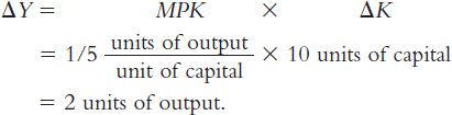
The marginal product of capital tells us how much output increases when capital increases by 1 unit. Therefore, when capital increases by ΔK units, output increases by approximately MPK × ΔK.16
For example, suppose that the marginal product of capital is 1/5; that is, an additional unit of capital increases the amount of output produced by one-fifth of a unit. If we increase the amount of capital by 10 units, we can compute the amount of additional output as follows:
271
By increasing capital by 10 units, we obtain 2 more units of output. Thus, we use the marginal product of capital to convert changes in capital into changes in output.
Increases in Labor Next, consider changes in labor. If the amount of labor increases by ΔL units, by how much does output increase? We answer this question the same way we answered the question about capital. The marginal product of labor MPL tells us how much output changes when labor increases by 1 unit—that is,
MPL = F(K, L + 1) − F(K, L).
Therefore, when the amount of labor increases by ΔL units, output increases by approximately MPL × ΔL.
For example, suppose that the marginal product of labor is 2; that is, an additional unit of labor increases the amount of output produced by 2 units. If we increase the amount of labor by 10 units, we can compute the amount of additional output as follows:
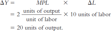
By increasing labor by 10 units, we obtain 20 more units of output. Thus, we use the marginal product of labor to convert changes in labor into changes in output.
Increases in Capital and Labor Finally, let’s consider the more realistic case in which both factors of production change. Suppose that the amount of capital increases by ΔK and the amount of labor increases by ΔL. The increase in output then comes from two sources: more capital and more labor. We can divide this increase into the two sources using the marginal products of the two inputs:
ΔY = (MPK × ΔK) + (MPL × ΔL).
The first term in parentheses is the increase in output resulting from the increase in capital; the second term in parentheses is the increase in output resulting from the increase in labor. This equation shows us how to attribute growth to each factor of production.
We now want to convert this last equation into a form that is easier to interpret and apply to the available data. First, with some algebraic rearrangement, the equation becomes17
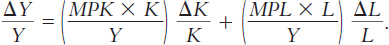
This form of the equation relates the growth rate of output, ΔY/Y, to the growth rate of capital, ΔK/K, and the growth rate of labor, ΔL/L.
272
Next, we need to find some way to measure the terms in parentheses in the last equation. In Chapter 3 we showed that the marginal product of capital equals its real rental price. Therefore, MPK × K is the total return to capital, and (MPK × K)/Y is capital’s share of output. Similarly, the marginal product of labor equals the real wage. Therefore, MPL × L is the total compensation that labor receives, and (MPL × L)/Y is labor’s share of output. Under the assumption that the production function has constant returns to scale, Euler’s theorem (which we discussed in Chapter 3) tells us that these two shares sum to 1. In this case, we can write
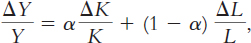
where α is capital’s share and (1 − α) is labor’s share.
This last equation gives us a simple formula for showing how changes in inputs lead to changes in output. It shows, in particular, that we must weight the growth rates of the inputs by the factor shares. Capital’s share in the United States is about 30 percent, that is, a = 0.30. Therefore, a 10 percent increase in the amount of capital (ΔK/K = 0.10) leads to a 3 percent increase in the amount of output (ΔY/Y = 0.03). Similarly, a 10 percent increase in the amount of labor (ΔL/L = 0.10) leads to a 7 percent increase in the amount of output (ΔY/Y = 0.07).
Technological Progress
So far in our analysis of the sources of growth, we have been assuming that the production function does not change over time. In practice, of course, technological progress improves the production function. For any given amount of inputs, we can produce more output today than we could in the past. We now extend the analysis to allow for technological progress.
We include the effects of the changing technology by writing the production function as
Y = AF(K, L),
where A is a measure of the current level of technology called total factor productivity. Output now increases not only because of increases in capital and labor but also because of increases in total factor productivity. If total factor productivity increases by 1 percent and if the inputs are unchanged, then output increases by 1 percent.
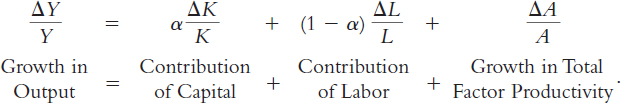
Allowing for a changing level of technology adds another term to our equation accounting for economic growth:
273
This is the key equation of growth accounting. It identifies and allows us to measure the three sources of growth: changes in the amount of capital, changes in the amount of labor, and changes in total factor productivity.
Because total factor productivity is not directly observable, it is measured indirectly. We have data on the growth in output, capital, and labor; we also have data on capital’s share of output. From these data and the growth-accounting equation, we can compute the growth in total factor productivity to make sure that everything adds up:
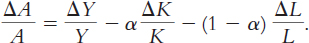
ΔA/A is the change in output that cannot be explained by changes in inputs. Thus, the growth in total factor productivity is computed as a residual—that is, as the amount of output growth that remains after we have accounted for the determinants of growth that we can measure directly. Indeed, ΔA/A is sometimes called the Solow residual, after Robert Solow, who first showed how to compute it.18
Total factor productivity can change for many reasons. Changes most often arise because of increased knowledge about production methods, so the Solow residual is frequently used as a measure of technological progress. Yet other factors, such as education and government regulation, can affect total factor productivity as well. For example, if higher public spending raises the quality of education, then workers may become more productive and output may rise, which implies higher total factor productivity. In another example, if government regulations require firms to purchase capital to reduce pollution or increase worker safety, then the capital stock may rise without any increase in measured output, which implies lower total factor productivity. Total factor productivity captures anything that changes the relation between measured inputs and measured output.
The Sources of Growth in the United States
Having learned how to measure the sources of economic growth, we now look at the data. Table 9-2 uses U.S. data to measure the contributions of the three sources of growth between 1948 and 2013.
TABLE 9-2
TABLE 9-2: Accounting for Economic Growth in the United States

This table shows that output in the non-farm business sector grew an average of 3.5 percent per year during this time. Of this 3.5 percent, 1.3 percent was attributable to increases in the capital stock, 1.0 percent to increases in the labor input, and 1.2 percent to increases in total factor productivity. These data show that increases in capital, labor, and productivity have contributed almost equally to economic growth in the United States.
274
Table 9-2 also shows that the growth in total factor productivity slowed substantially during the period from 1972 to 1995. Before 1972, total factor productivity grew at 1.8 percent per year; after 1972, it grew at only 0.5 percent per year. Accumulated over many years, even a small change in the rate of growth has a large effect on economic well-being. Real income in the United States in 1995 and beyond was about 35 percent lower than it would have been had productivity growth remained at its previous level.
CASE STUDY
The Slowdown in Productivity Growth
Why did the slowdown in productivity growth around 1972 occur? There are many hypotheses to explain this adverse phenomenon. Here are four of them.
Measurement Problems One possibility is that the productivity slowdown did not really occur and that it shows up in the data because the data are flawed. As you may recall from Chapter 2, one problem in measuring inflation is correcting for changes in the quality of goods and services. The same issue arises when measuring output and productivity. For instance, if technological advance leads to more computers being built, then the increase in output and productivity is easy to measure. But if technological advance leads to faster computers being built, then output and productivity have increased, but that increase is more subtle and harder to measure. Government statisticians try to correct for changes in quality, but despite their best efforts, the resulting data are far from perfect.
275
Unmeasured quality improvements mean that our standard of living is rising more rapidly than the official data indicate. This issue should make us suspicious of the data, but by itself it cannot explain the productivity slowdown. To explain a slowdown in growth, one must argue that the measurement problems got worse. There is some indication that this might be so. As history passes, fewer people work in industries with tangible and easily measured output, such as agriculture, and more work in industries with intangible and less easily measured output, such as medical services. Yet few economists believe that measurement problems were the full story.
Oil Prices When the productivity slowdown began around 1973, the obvious hypothesis to explain it was the large increase in oil prices caused by the actions of the OPEC oil cartel. The primary piece of evidence was the timing: productivity growth slowed at the same time that oil prices skyrocketed. Over time, however, this explanation has appeared less likely. One reason is that the accumulated shortfall in productivity seems too large to be explained by an increase in oil prices; petroleum-based products are not that large a fraction of a typical firm’s costs. In addition, if this explanation were right, productivity should have sped up when political turmoil in OPEC caused oil prices to plummet in 1986. Unfortunately, that did not happen.
Worker Quality Some economists suggest that the productivity slowdown might have been caused by changes in the labor force. In the early 1970s, the large baby-boom generation started leaving school and taking jobs. At the same time, changing social norms encouraged many women to leave full-time housework and enter the labor force. Both of these developments lowered the average level of experience among workers, which in turn lowered average productivity.
Other economists point to changes in worker quality as gauged by human capital. Although the educational attainment of the labor force continued to rise throughout this period, it was not increasing as rapidly as it had in the past. Moreover, declining performance on some standardized tests suggests that the quality of education was declining. If so, this could explain slowing productivity growth.
The Depletion of Ideas Still other economists suggest that in the early 1970s the world started running out of new ideas about how to produce, pushing the economy into an age of slower technological progress. These economists often argue that the anomaly is not in the period since 1970 but in the preceding two decades. In the late 1940s, the economy had a large backlog of ideas that had not been fully implemented because of the Great Depression of the 1930s and World War II in the first half of the 1940s. After the economy used up this backlog, the argument goes, a slowdown in productivity growth was likely. Indeed, although the growth rates after 1972 were disappointing compared to those of the 1950s and 1960s, they were not lower than average growth rates from 1870 to 1950.
276
As any good doctor will tell you, sometimes a patient’s illness goes away on its own, even if the doctor has failed to come up with a convincing diagnosis and remedy. This seems to be the outcome of the productivity slowdown. In the middle of the 1990s, productivity growth accelerated. Most observers attribute this acceleration to advances in computers and information technology.19 
CASE STUDY
Growth in the East Asian Tigers
Among the most spectacular growth experiences in recent history have been those of the “Tigers” of East Asia: Hong Kong, Singapore, South Korea, and Taiwan. From 1966 to 1990, while real income per person was growing about 2 percent per year in the United States, it grew more than 7 percent per year in each of these countries. In the course of a single generation, real income per person increased fivefold, moving the Tigers from among the world’s poorest countries to among the richest. (In the late 1990s, a period of pronounced financial turmoil tarnished the reputations of some of these economies. But this short-run problem, which we examine in a Case Study in Chapter 13, doesn’t come close to reversing the spectacular long-run growth that the Asian Tigers have experienced.)
What accounts for these growth miracles? Some commentators have argued that the success of these four countries is hard to reconcile with basic growth theory, such as the Solow growth model, which takes technology as growing at a constant, exogenous rate. They have suggested that these countries’ rapid growth is explained by their ability to imitate foreign technologies. By adopting technology developed abroad, the argument goes, these countries managed to improve their production functions substantially in a relatively short period of time. If this argument is correct, these countries should have experienced unusually rapid growth in total factor productivity.
One study shed light on this issue by examining in detail the data from these four countries. The study found that their exceptional growth can be traced to large increases in measured factor inputs: increases in labor-force participation, increases in the capital stock, and increases in educational attainment. In South Korea, for example, the investment–GDP ratio rose from about 5 percent in the 1950s to about 30 percent in the 1980s; the percentage of the working population with at least a high school education went from 26 percent in 1966 to 75 percent in 1991.
Once we account for growth in labor, capital, and human capital, little of the growth in output is left to explain. None of these four countries experienced unusually rapid growth in total factor productivity. Indeed, the average growth in total factor productivity in the East Asian Tigers was almost exactly the same as in the United States. Thus, although these countries’ rapid growth was truly impressive, it is easy to explain using the tools of basic growth theory.20
277
The Solow Residual in the Short Run
When Robert Solow introduced his famous residual, his aim was to shed light on the forces that determine technological progress and economic growth in the long run. But economist Edward Prescott has looked at the Solow residual as a measure of technological change over shorter periods of time. He concludes that fluctuations in technology are a major source of short-run changes in economic activity.
Figure 9-2 shows the Solow residual and the growth in output using annual data for the United States during the period 1960 to 2013. Notice that the Solow residual fluctuates substantially. If Prescott’s interpretation is correct, then we can draw conclusions from these short-run fluctuations, such as that technology worsened in 1982 and improved in 1984. Notice also that the Solow residual moves closely with output: in years when output falls, technology tends to worsen. In Prescott’s view, this fact implies that recessions are driven by adverse shocks to technology. The hypothesis that technological shocks are the driving force behind short-run economic fluctuations, and the complementary hypothesis that monetary policy has no role in explaining these fluctuations, is the foundation for an approach called real-business-cycle theory.
FIGURE 9-2

278
Prescott’s interpretation of these data is controversial, however. Many economists believe that the Solow residual does not accurately represent changes in technology over short periods of time. The standard explanation of the cyclical behavior of the Solow residual is that it results from two measurement problems.
First, during recessions, firms may continue to employ workers they do not need so that they will have these workers on hand when the economy recovers. This phenomenon, called labor hoarding, means that labor input is overestimated in recessions because the hoarded workers are probably not working as hard as usual. As a result, the Solow residual is more cyclical than the available production technology. In a recession, productivity as measured by the Solow residual falls even if technology has not changed simply because hoarded workers are sitting around waiting for the recession to end.
Second, when demand is low, firms may produce things that are not easily measured. In recessions, workers may clean the factory, organize the inventory, get some training, and do other useful tasks that standard measures of output fail to include. If so, then output is underestimated in recessions, which would also make the measured Solow residual cyclical for reasons other than technology.
Thus, economists can interpret the cyclical behavior of the Solow residual in different ways. Some economists point to the low productivity in recessions as evidence for adverse technology shocks. Others believe that measured productivity is low in recessions because workers are not working as hard as usual and because more of their output is not measured. Unfortunately, there is no clear evidence on the importance of labor hoarding and the cyclical mismeasurement of output. Therefore, different interpretations of Figure 9-2 persist.21
279