167

APPENDIX

The Open Economy in the Very Long Run

The main body of this chapter involves the small-open-economy version of the Chapter 3 material. In this appendix, we consider the small-open-economy version of some of the material that is in Chapters 7 and 8. The closed-economy analysis focuses on how saving leads to capital accumulation and higher living standards in the future. In the open setting, the assumption of perfect capital mobility makes the quantity of capital employed within the domestic economy independent of national saving. Thus, with both the capital stock and the labour force determined exogenously, real GDP cannot be increased by national saving. But GNP is affected. With higher national saving, the level of foreign indebtedness can be reduced. Higher consumption is possible in the long run as a result of the corresponding reduction in interest payment obligations to foreigners. The purpose of this appendix is to explain this process in detail.

In the main part of this chapter, we did not need to distinguish between the trade balance and the current account balance. But now it is helpful to do so. To that end, we divide net exports into two components: the net sale of goods and nonfinancial services to the rest of the world (the trade balance) minus the net interest payments Canadians make each year to foreigners to pay for that year’s lending services that were imported. Letting NX stand for the first component, and letting Z and r denote the level of foreign debt and the interest rate involved on that debt, the overall current account balance is NX – rZ. As before, the excess of national saving over domestic investment, S – I, must equal the current account balance, so in this more detailed specification,

S – I = NX – rZ.

Another way to appreciate this relationship is to note that, when the distinction between GNP and GDP is not ignored for simplicity, private saving is GNP – T – C. Since GNP = GDP – rZ, and since GDP = C + I + G + NX, these two relationships imply S– I = NX – rZ.

National wealth is the excess of our assets over our debt, that is, K – Z. Since saving is the increase in national wealth (S = ΔK – ΔZ), and since investment is the change in the capital stock (I = ΔK), the fundamental equation given above can be re-expressed as foreign debt accumulation identity:

ΔZ = rZ– NX.

This equation states that our debt to foreigners increases whenever interest payment obligations on the pre-existing debt for that period, rZ, exceed what we earn from our net-export sales from other items that period, NX.

168

A long-run equilibrium exists when the foreign debt-to-GDP ratio, Z/Y, is constant. Defining the GDP growth rate as n (ΔY/Y = n), long-run equilibrium requires ΔZ/Z = n, or ΔZ = nZ. Substituting this balanced growth requirement into the accumulation identity, we have the long-run equilibrium condition

(r – n)Z = NX.

Before we use these two relationships—the accumulation identity to determine outcomes initially and the equilibrium condition to determine outcomes eventually—we clarify two things. First, this analysis takes both r and n as exogenous variables. The interest rate is determined in the rest of the world via the assumption of perfect capital mobility. The growth rate of the effective labour force is exogenous, as in the Solow model (explained in Chapter 7). The second thing to bear in mind is that the interest rate (the marginal product of capital) exceeds the growth rate, so (r −n) is positive. We will learn why this is the case when we discover that Canada has a smaller capital labour ratio than the Golden Rule value (Chapter 7).

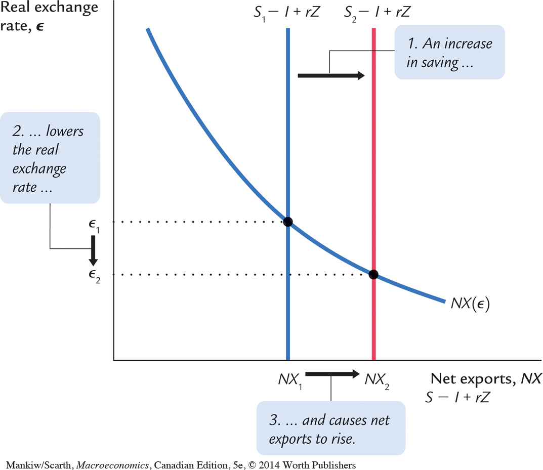
We are now in a position to see how our analysis of fiscal policy can be enriched by considering these longer-term relationships. The main initiative of the Canadian government during the 1990s was deficit reduction—accomplished primarily by cuts in government spending. Thus, in Figure 5-16 we explore the effect of a cut in government spending. Initially, the analysis duplicates what we learned when studying Figure 5-10; the only difference here is that spending is decreased, not increased. The graph shows the key implication of fiscal retrenchment—that net exports rise.

169

We can now appreciate the longer-term implication of this rise in net exports. Consider each term in the foreign debt accumulation identity. Since the preexisting level of Z is determined by whatever history took place before this fiscal policy, and since r is exogenous (equal to r*), higher NX implies lower ΔZ. Thus a higher level of net exports initially makes our foreign debt obligations shrink.

What are the long-term implications of lower debt? This question can be answered by considering the full equilibrium condition. Given that (r – n) is positive and that Z is eventually lower, the left-hand side of the equilibrium condition must be smaller. This means that, eventually, NX must be smaller too. So, as time passes, net exports must move in the opposite direction from what occurs initially.

To appreciate why this occurs, we must realize that the consumption function requires an amendment to make it applicable in this longer-term setting. In particular, to be both realistic and consistent with the optimization-based theories of consumption, which are introduced in Chapter 17, we must assume that consumption depends on both disposable income and wealth (and therefore foreign indebtedness: C = C(Y – T, Z)). Since households cannot afford to consume as much when they are heavily in debt, we know that consumption depends inversely on foreign debt. As a result, since national saving is (Y – C – G), S depends positively on Z. Figure 5-17 shows the result of this dependence. While the cut in G increases the public sector component of national savings and so shifts the net savings line to the right initially, the falling level of foreign debt induces a gradual drop in the private sector component of national savings; so the net savings line drifts back to the left. The algebraic version of the long-run equilibrium condition indicates that this process is not complete until a point like C in Figure 5-17 is reached.

170

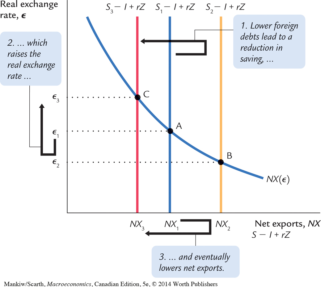
It is instructive to summarize the time path of the real exchange rate following fiscal retrenchment. That response is from point A to B initially, and then from B to C later on. Thus, the analysis predicts that the domestic currency falls in value initially, but that this outcome is reversed and that the exchange rate rises eventually. Many commentators on exchange-rate developments appear to reason in a way that does not reflect this “overshoot” in the real exchange rate. For example, it is usually presumed that tight fiscal policy—since it involves “getting our fiscal house in order”—causes a straightforward appreciation of our currency. The limited success of empirical studies on exchange-rate determination may have a lot to do with the fact that the reversal and overshoot features in the theory are often precluded in the way statistical studies are performed.

But we should not be too critical of the empirical work. On balance, our theory suggests that Canada’s real exchange rate (vis-à-vis the U.S. dollar) should have fallen during the 1970–2000 time period—both because we had a looser fiscal policy and because we have a more resource-based economy than do the Americans. As a result of our increased dependence on the resource sectors, the demand for our net exports was more affected by the drop in the demand for primary commodities in world markets. In addition to these key determinants of the real exchange rate, there was additional downward pressure on our nominal exchange rate, since—until the last few years of the century—we had higher inflation. It has been estimated that of the 30-cent fall in the Canadian dollar over 30 years (from par with the U.S. currency in 1970), roughly 10 cents can be attributed to each of these three factors.

Since 2000, there has been a world commodity price boom (which has increased the demand for Canadian exports) and a major reversal in Canadian-American fiscal policy. Until 2009, we have had large government budget surpluses, while Americans have recorded record budget deficits. As our analysis predicts, the long-run implications of these developments is a rising Canadian dollar (a rising Canada-U.S. dollar exchange rate). It is reassuring that the analysis is so applicable for interpreting economic history.

As we have seen, anything that raises national saving leads to higher living standards in the longer term. Often the government tries to implement this strategy by offering tax breaks for saving. This policy is criticized on the grounds that only the rich can afford to save, so the poor do not share the benefits. Proponents of this approach answer this criticism by arguing that the benefits “trickle down” indirectly to those on lower incomes, so everyone benefits indirectly after all. Let us assess the validity of this claim—first in a closed-economy setting as a base for comparison, and then in an open setting.

171

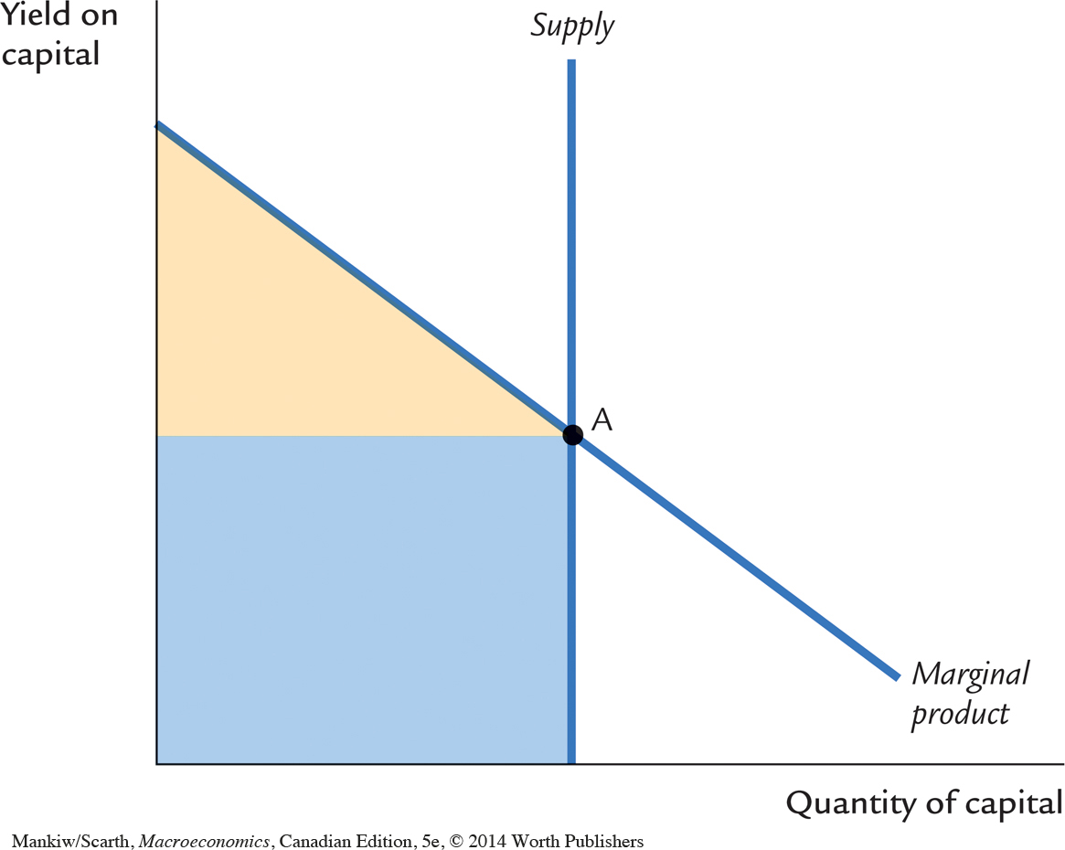
Figure 5-18 shows the diminishing marginal product of capital relationship. Initially, the quantity of capital is given by the position of the supply curve in Figure 5-18. The equilibrium return on capital (the interest rate) is given by the intersection of supply and demand in Figure 5-18: the height of point A. The total earnings of capital (the yield per unit times number of units) is given by the light blue rectangle. Since the area under the marginal product curve is total output, labourers receive the light beige triangle, and total GDP is the sum of capital’s rectangle and labour’s triangle. To assess the trickle-down theory, let us assume that capital owners are “rich,” while labourers are “poor.” We now consider whether an increase in national saving helps labour.

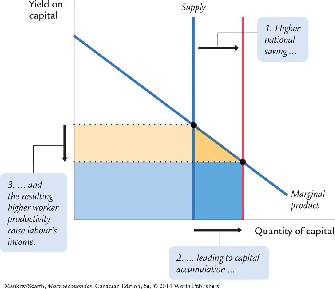
In a closed economy, higher saving means more investment, which leads eventually to a larger capital stock. We show that higher capital stock by moving the supply curve to the right in Figure 5-19. GDP has increased by an amount equal to the trapezoid of dark shaded regions on the right (labour gets the beige part, capital gets the blue part). Labour’s total income has increased by the trapezoid created by the two horizontal dotted lines (both the light and dark beige regions in Figure 5-19). We can conclude that, even if labour does not benefit in any direct way from the tax cut (or other initiative used to stimulate saving), there appears to be solid support for the trickle-down view. The intuition behind this conclusion is that each worker has more capital with which to work and so receives higher wages.

172

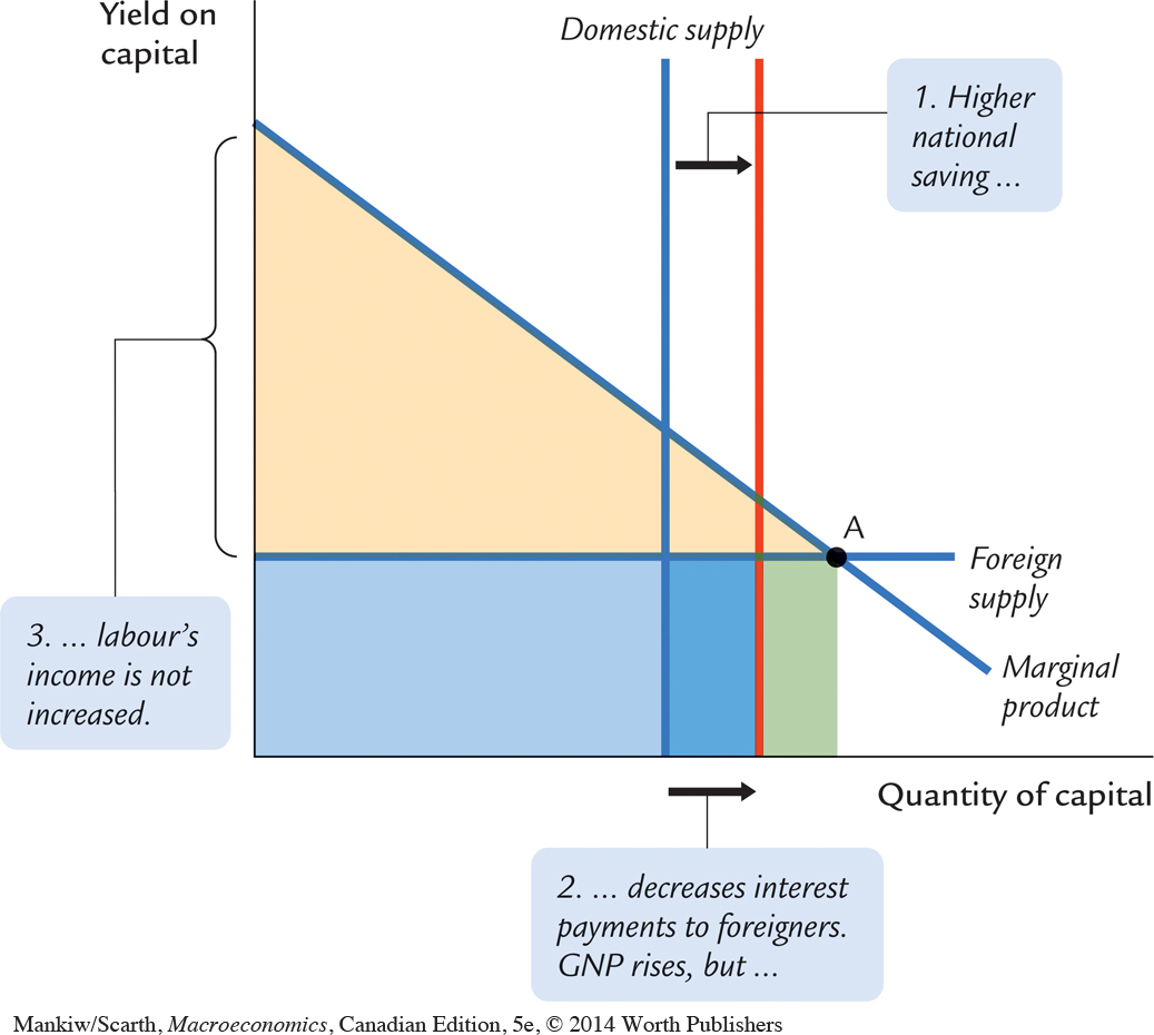
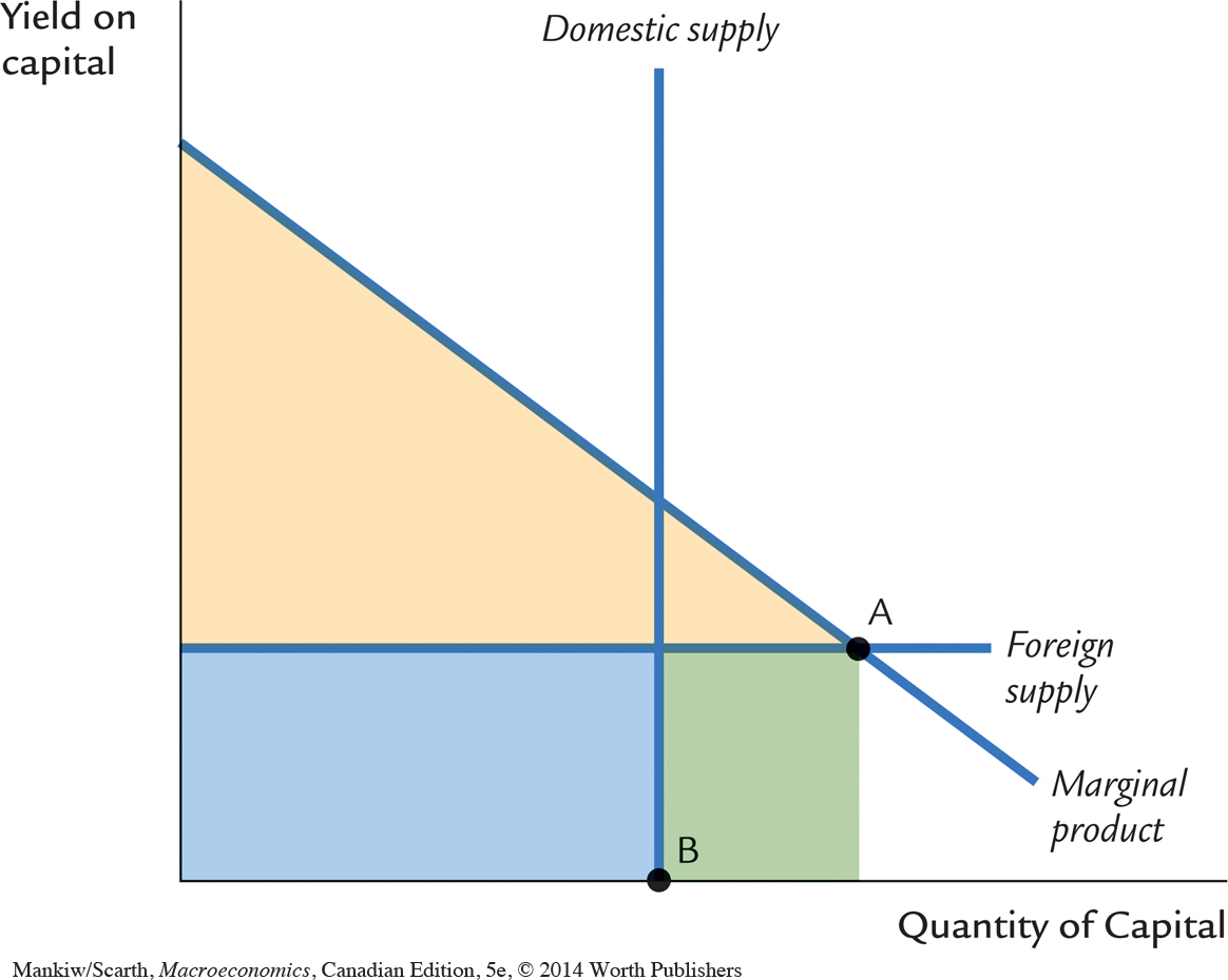
Does this conclusion carry over to a small open economy? The initial situation in this case is shown in Figure 5-20. With perfect capital mobility, there is a perfectly elastic supply of capital (from the rest of the world) at the prevailing world yield on capital. Supply and demand for capital intersect at point A, so GDP is determined by the trapazoid formed by the perpendicular dropped from point A. Capital owners receive the lower rectangles, while labour receives the upper, beige triangle. The vertical line in Figure 5-20 indicates what part of the capital is owned by domestic residents. Given the position of this line, we have assumed that domestic residents own the proportion of the capital that is denoted by point B. Thus, domestic capitalists receive the light blue rectangle and foreigners receive the green rectangle. Since GNP is GDP minus income going to foreigners, GNP is the entire coloured area minus this green region.

As in the closed economy, the results of higher saving are shown by shifting the vertical line to the right—as illustrated in Figure 5-21. In this case, the location of point A is unaffected, so GDP is no different. Wealth still increases, because the higher saving allows domestic residents to reduce foreign debt. The smaller interest payment obligation to foreigners is shown by the fact that the green region is smaller in Figure 5-21. Thus GNP increases, even though GDP does not. Since GNP is national income, the aggregate effect is much the same even if the reason for it differs. Domestic residents are better off because they have a smaller mortgage to finance, not because workers have more capital to work with. However, the distribution of the benefit is very different. Because workers have no more capital, wages are no higher, and this is why the size of labour’s beige triangle is not affected. We conclude that there is not strong support for trickle down in a small open economy setting.

173