8.1 Technological Progress in the Solow Model
So far, our model has assumed an unchanging relationship between the inputs of capital and labour and the output of goods and services. Yet the model can be modified to include exogenous technological progress, which over time expands society’s production capabilities.
The Efficiency of Labour
To incorporate technological progress, we must return to the production function that relates total capital K and total labour L to total output Y. Thus far, the production function has been
Y = F(K, L).
We now write the production function as
Y = F(K, L × E),
where E is a new (and somewhat abstract) variable called the efficiency of labour. The efficiency of labour is meant to reflect society’s knowledge about production methods: as the available technology improves, the efficiency of labour rises, and each hour of work contributes more to the production of goods and services. For instance, the efficiency of labour rose when assembly-line production transformed manufacturing in early twentieth century, and it rose again when computerization was introduced in the the late twentieth century. The efficiency of labour also rises when there are improvements in the health, education, or skills of the labour force, and when institutions develop that better allow individual initiative to be harnessed.
The term L × E can be interpreted as measuring the effective number of workers. It takes into account the number of actual workers L and the efficiency of each worker E. In other words, L measures the number of workers in the labour force, whereas L × E measures both the workers and the technology with which the typical worker is equipped. This new production function states that total output Y depends on the number of units of capital K and on the effective number of workers, L × E. The essence of this approach to modeling technological progress is that increases in the efficiency of labour E are analogous to increases in the labour force L. Suppose, for example, that an advance in production methods makes the efficiency of labour E double between 1980 and 2010. This means that a single worker in 2010 is, in effect, as productive as two workers were in 1980. That is, even if the actual number of workers (L) stays the same from 1980 to 2010, the effective number of workers (L × E) doubles, and the economy benefits from an increased production of goods and services.
The simplest assumption about technological progress is that it causes the efficiency of labour E to grow at some constant rate g. For example, if g =0.02, then each unit of labour becomes 2 percent more efficient each year: output increases as if the labour force had increased by 2 percent more than it really did. This form of technological progress is called labour augmenting, and g is called the rate of labour-augmenting technological progress. Because the labour force L is growing at rate n, and the efficiency of each unit of labour E is growing at rate g, the effective number of workers L × E is growing at rate n + g.
The Steady State with Technological Progress
Because technological progress is modeled here as labour augmenting, it fits into the Solow model much the same as population growth does. Although technological progress does not cause the actual number of workers to increase, each worker in effect comes with more units of labour over time. Thus, technological progress causes the effective number of workers to increase. As a result, the analytic tools we used in Chapter 7 to study the Solow model with population growth are easily adapted to study the Solow model with labour-augmenting technological progress.
We begin by reconsidering our notation. Previously, when there was no technological progress, we analyzed the economy in terms of quantities per worker; now we can generalize that approach by analyzing the economy in terms of quantities per effective worker. We now let k = K/(L × E) stand for capital per effective worker, and y = Y/(L × E) stand for output per effective worker. With these definitions, we can again write y = f(k).
Our analysis of the economy proceeds just as it did when we examined population growth. The equation showing the evolution of k over time becomes
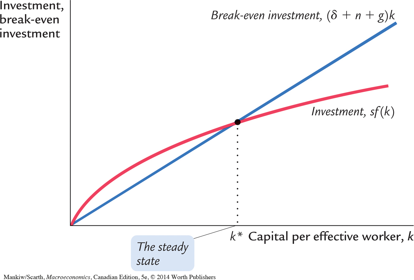
Δk = sf(k) – (δ + n + g)k.
As before, the change in the capital stock Δk equals investment sf(k) minus break-even investment (δ + n + g)k. Now, however, because k = K/EL, break-even investment includes three terms: to keep k constant, δk is needed to replace depreciating capital, nk is needed to provide capital for new workers, and gk is needed to provide capital for the new “effective workers” created by technological progress.1
As shown in Figure 8-1, the inclusion of technological progress does not substantially alter our analysis of the steady state. There is one level of k, denoted k*, at which capital per effective worker and output per effective worker are constant. As before, this steady state represents the long-run equilibrium of the economy.
The Effects of Technological Progress
Table 8-1 shows how four key variables behave in the steady state with technological progress. As we have just seen, capital per effective worker k is constant in the steady state. Because y = (k), output per effective worker is also constant. These quantities per effective worker are steady in the steady state.
| Variable | Symbol | Steady-State Growth Rate |
| Capital per effective worker | k = K/(E × L) | 0 |
| Output per effective worker | y = Y/(E × L) = f(k) | 0 |
| Output per worker | Y/L = y × E | g |
| Total output | Y = y × (E × L) | n + g |
From this information, we can also infer what’s happening to variables that are not expressed in per-effective-worker units. For instance, consider output per actual worker Y/L = y × E. Because y is constant in the steady state and E is growing at rate g, output per worker must also be growing at rate g in the steady state. Similarly, the economy’s total output is Y = y × (E × L). Because y is constant in the steady state, E is growing at rate g, and L is growing at rate n, total output grows at rate  in the steady state.
With the addition of technological progress, our model can finally explain the sustained increases in standards of living that we observe. That is, we have shown that technological progress can lead to sustained growth in output per worker. By contrast, a high rate of saving leads to a high rate of growth only until the steady state is reached. Once the economy is in steady state, the rate of growth of output per worker depends only on the rate of technological progress. According to the Solow model, only technological progress can explain sustained growth and persistently rising living standards.
The introduction of technological progress also modifies the criterion for the Golden Rule. The Golden Rule level of capital is now defined as the steady state that maximizes consumption per effective worker. Following the same arguments that we have used before, we can show that steady-state consumption per effective worker is
c* = f(k*) – (δ + n + g)k*.
Steady-state consumption is maximized if
MPK = δ + n + g,
or
MPK – δ = n + g.
That is, at the Golden Rule level of capital, the net marginal product of capital, MPK – δ, equals the rate of growth of total output, n + g. Because actual economies experience both population growth and technological progress, we must use this criterion to evaluate whether they have more or less capital than they would at the Golden Rule steady state.