13.2 Inflation, Unemployment, and the Phillips Curve
Two goals of economic policymakers are low inflation and low unemployment, but often these goals conflict. Suppose, for instance, that policymakers were to use monetary or fiscal policy to expand aggregate demand. This policy would move the economy along the short-run aggregate supply curve to a point of higher output and a higher price level. (Figure 13-2 shows this as the change from point A to point B.) Higher output means lower unemployment, because firms employ more workers when they produce more. A higher price level, given the previous year’s price level, means higher inflation. Thus, when policymakers move the economy up along the short-run aggregate supply curve, they reduce the unemployment rate and raise the inflation rate. Conversely, when they contract aggregate demand and move the economy down the short-run aggregate supply curve, unemployment rises and inflation falls.
This tradeoff between inflation and unemployment, called the Phillips curve, is our topic in this section. As we have just seen (and will derive more formally in a moment), the Phillips curve is a reflection of the short-run aggregate supply curve: as policymakers move the economy along the short-run aggregate supply curve, unemployment and inflation move in opposite directions. The Phillips curve is a useful way to express aggregate supply because inflation and unemployment are such important measures of economic performance.
Deriving the Phillips Curve from the Aggregate Supply Curve
The Phillips curve in its modern form states that the inflation rate depends on three forces:
Expected inflation
The deviation of unemployment from the natural rate, called cyclical unemployment
Supply shocks.
These three forces are expressed in the following equation:
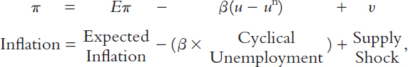
where β is a parameter measuring the response of inflation to cyclical unemployment. Notice that there is a minus sign before the cyclical unemployment term: other things equal, higher unemployment is associated with lower inflation.
Where does this equation for the Phillips curve come from? Although it may not seem familiar, we can derive it from our equation for aggregate supply. To see how, write the aggregate supply equation as
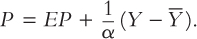
With one addition, one subtraction, and one substitution, we can transform this equation into the Phillips curve—a relationship between inflation and unemployment.
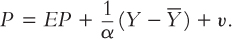
Here are the three steps. First, add to the right-hand side of the equation a supply shock v to represent exogenous events (such as a change in world oil prices) that alter the price level and shift the short-run aggregate supply curve:
Next, to go from the price level to inflation rates, subtract last year’s price level P–1 from both sides of the equation to obtain
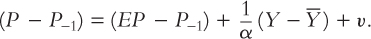
The term on the left-hand side, P – P–1, is the difference between the current price level and last year’s price level, which is inflation π.6 The term on the right-hand side, EP – P–1, is the difference between the expected price level and last year’s price level, which is expected inflation Eπ. Therefore, we can replace P – P–1 with π and EP – P–1 with Eπ:
Third, to go from output to unemployment, recall from Chapter 2 that Okun’s law gives a relationship between these two variables. One version of Okun’s law states that the deviation of output from its natural level is inversely related to the deviation of unemployment from its natural rate; that is, when output is higher than the natural level of output, unemployment is lower than the natural rate of unemployment. We can write this as
Using this Okun’s law relationship, we can substitute –β(u – un) for (1/α)(Y– ) in the previous equation to obtain:
π= Eπ –β(u – un) + v.
Thus, we can derive the Phillips curve equation from the aggregate supply equation.
All this algebra is meant to show one thing: the Phillips curve equation and the short-run aggregate supply equation represent essentially the same macroeconomic ideas. In particular, both equations show a link between real and nominal variables that causes the classical dichotomy (the theoretical separation of real and nominal variables) to break down in the short run. According to the short-run aggregate supply equation, output is related to unexpected movements in the price level. According to the Phillips curve equation, unemployment is related to unexpected movements in the inflation rate. The aggregate supply curve is more convenient when we are studying output and the price level, whereas the Phillips curve is more convenient when we are studying unemployment and inflation. But we should not lose sight of the fact that the Phillips curve and the aggregate supply curve are merely two sides of the same coin.
FYI
The History of the Modern Phillips Curve
The Phillips curve is named after New Zealand-born economist A. W. Phillips. In 1958 Phillips observed a negative relationship between the unemployment rate and the rate of wage inflation in data for the United Kingdom.7 The Phillips curve that economists use today differs in three ways from the relationship Phillips examined.
First, the modern Phillips curve substitutes price inflation for wage inflation. This difference is not crucial, because price inflation and wage inflation are closely related. In periods when wages are rising quickly, prices are rising quickly as well.
Second, the modern Phillips curve includes expected inflation. This addition is due to the work of Milton Friedman and Edmund Phelps. In developing early versions of the imperfect information model in the 1960s, these two economists emphasized the importance of expectations for aggregate supply.
Third, the modern Phillips curve includes supply shocks. Credit for this addition goes to OPEC, the Organization of Petroleum Exporting Countries. In the 1970s OPEC caused large increases in the world price of oil, which made economists more aware of the importance of shocks to aggregate supply.
Adaptive Expectations and Inflation Inertia
To make the Phillips curve useful for analyzing the choices facing policymakers, we need to specify what determines expected inflation. A simple and often plausible assumption is that people form their expectations of inflation based on recently observed inflation. This assumption is called adaptive expectations. For example, suppose that people expect prices to rise this year at the same rate as they did last year. Then expected inflation Eπ equals last year’s inflation π–1:
Eπ = π–1.
In this case, we can write the Phillips curve as
π = π–1 – β(u – un) +v,
which states that inflation depends on past inflation, cyclical unemployment, and a supply shock. When the Phillips curve is written in this form, the natural rate of unemployment is sometimes called the Nonaccelerating Inflation Rate of Unemployment (NAIRU).
The first term in this form of the Phillips curve, π–1, implies that inflation has inertia. That is, like an object moving through space, inflation keeps going unless something acts to stop it. In particular, if unemployment is at the NAIRU and if there are no supply shocks, the price level will continue to rise at the rate it has been rising. This inertia arises because past inflation influences expectations of future inflation and because these expectations influence the wages and prices that people set. Robert Solow captured the concept of inflation inertia well when, during the high inflation of the 1970s, he wrote, “Why is our money ever less valuable? Perhaps it is simply that we have inflation because we expect inflation, and we expect inflation because we’ve had it.”
In the model of aggregate supply and aggregate demand, inflation inertia is interpreted as persistent upward shifts in both the aggregate supply curve and the aggregate demand curve. Consider first aggregate supply. If prices have been rising quickly, people will expect them to continue to rise quickly. Because the position of the short-run aggregate supply curve depends on the expected price level, the short-run aggregate supply curve will shift upward over time. It will continue to shift upward until some event, such as a recession or a supply shock, changes inflation and thereby changes expectations of inflation.
The aggregate demand curve must also shift upward to confirm the expectations of inflation. Most often, the continued rise in aggregate demand is due to persistent growth in the money supply. If the Bank of Canada suddenly halted money growth, aggregate demand would stabilize, and the upward shift in aggregate supply would cause a recession. The high unemployment in the recession would reduce inflation and expected inflation, causing inflation inertia to subside.
Two Causes of Rising and Falling Inflation
The second and third terms in the Phillips curve equation show the two forces that can change the rate of inflation.
The second term, β(u – un), shows that cyclical unemployment—the deviation of unemployment from its natural rate—exerts upward or downward pressure on inflation. Low unemployment pulls the inflation rate up. This is called demand-pull inflation because high aggregate demand is responsible for this type of inflation. High unemployment pulls the inflation rate down. The parameter β measures how responsive inflation is to cyclical unemployment.
The third term, v, shows that inflation also rises and falls because of supply shocks. An adverse supply shock, such as the rise in world oil prices in the 1970s, implies a positive value of v and causes inflation to rise. This is called cost-push inflation because adverse supply shocks are typically events that push up the costs of production. A beneficial supply shock, such as the oil glut that led to a fall in oil prices in the 1980s, makes v negative and causes inflation to fall.
The Short-Run Tradeoff Between Inflation and Unemployment
Consider the options the Phillips curve gives to a policymaker who can influence aggregate demand with monetary or fiscal policy. At any moment, expected inflation and supply shocks are beyond the policymaker’s immediate control. Yet, by changing aggregate demand, the policymaker can alter output, unemployment, and inflation. The policymaker can expand aggregate demand to lower unemployment and raise inflation. Or the policymaker can depress aggregate demand to raise unemployment and lower inflation.
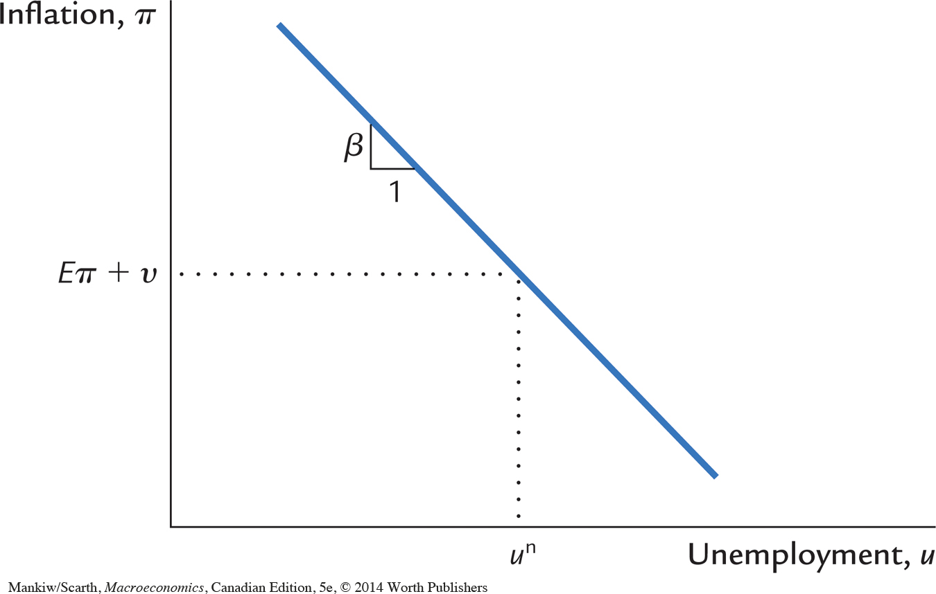
Figure 13-3 plots the Phillips curve equation and shows the short-run tradeoff between inflation and unemployment. When unemployment is at its natural rate (u = un), inflation depends on expected inflation and the supply shock (π = Eπ + v). The parameter β determines the slope of the tradeoff between inflation and unemployment. In the short run, for a given level of expected inflation, policymakers can manipulate aggregate demand to choose any combination of inflation and unemployment on this curve, called the short-run Phillips curve.
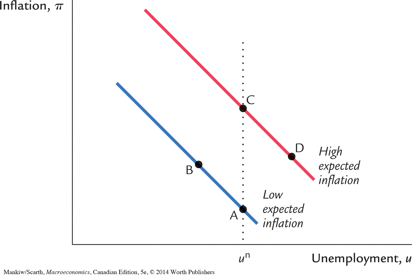
Notice that the position of the short-run Phillips curve depends on the expected rate of inflation. If expected inflation rises, the curve shifts upward, and the policymaker’s tradeoff becomes less favourable: inflation is higher for any level of unemployment. Figure 13-4 shows how the tradeoff depends on expected inflation.
Because people adjust their expectations of inflation over time, the tradeoff between inflation and unemployment holds only in the short run. The policymaker cannot keep inflation above expected inflation (and thus unemployment below its natural rate) forever. Eventually, expectations adapt to whatever inflation rate the policymaker has chosen. In the long run, the classical dichotomy holds, unemployment returns to its natural rate, and there is no tradeoff between inflation and unemployment.
To follow this process explicitly, assume that the economy is initially at point A in Figure 13-4—a point at which actual and expected inflation coincide. Then, assume that expansionary monetary or fiscal policy is used to move the economy from point A to point B. The short-run tradeoff is operating; there are lower unemployment and higher inflation. But the economy cannot stay at point B since it involves actual inflation being greater than peoples’ expectations of inflation. As individuals revise their expectations upward, there is a tendency for the point showing the economy’s outcome to move up in Figure 13-4. Often, in this situation, the government begins to contract aggregate demand—now that it realizes that the inflationary consequences of its previous policy are larger than first assumed. This reaction creates a tendency for the point showing the economy’s outcome to move back to the right in Figure 13-4. The net effect of these two tendencies—the upward revision in inflationary expectations and the backing off of aggregate demand policy—is an upward-sloping move from point B to point C. At this stage, there is not a tradeoff; both unemployment and inflation are rising.
Point C is sustainable in the long run. Unemployment has returned to the natural rate and actual and expected inflation are consistent (they are both high). When the government wants to fight inflation, contractionary monetary and fiscal policy move the outcome from point C to point D. Again we see a short-run tradeoff—inflation falling but unemployment rising. But because actual inflation is less than expected inflation at point D, expectations are revised down. The economy spends a long time at point D if people are slow to adjust expectations, and there will be a significant sacrifice involved in fighting inflation—a prolonged period of high unemployment.
We can summarize the options for policymakers quite simply. There is a short-run tradeoff between unemployment and inflation, and this fact is indicated by the set of negatively sloped relationships in Figure 13-4. But there is no long-run relationship between unemployment and inflation, and this is indicated by the fact that all long-run-sustainable points in Figure 13-4 occur on a vertical line (denoted by AC). Another way to appreciate the temporary nature of the short-run tradeoff is to focus on the fact that it describes a relationship between cyclical unemployment and inflation. Because, by definition, the average level of cyclical unemployment is zero, that average level cannot be dependent on the level of inflation. If policymakers wish to lower the long-run average level of unemployment (that is, if they wish to lower structural unemployment—the natural rate), they must not look to monetary policy. Instead they must rely on the fiscal policies that were explored in Chapter 6. If the natural unemployment rate can be lowered by such policies, the increased level of employment would raise the natural level of output . As a result, Okun’s law would be unaffected: the output gap would still be related to the unemployment gap. Graphically, then, a reduction in the natural unemployment rate shifts both the vertical long-run Phillips curve and the family of short-run Phillips (with their negative slope unaltered) to the left.
CASE STUDY
Inflation and Unemployment in Canada
Figure 13-5 depicts the history of inflation and unemployment in Canada since 1956. We see that the pre-1970 observations (all squares without a date label) are well summarized by the negatively sloped Phillips curve. During this period, there were few large supply shocks, and the government never allowed aggregate demand to expand so much that a sustained inflation developed. As a result, inflationary expectations played little role.
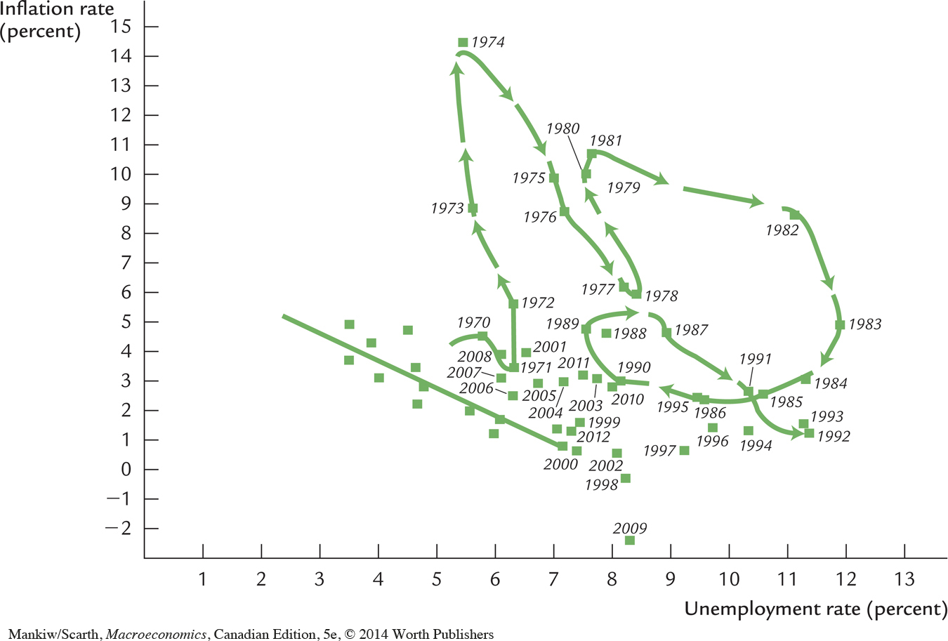
Then, in the 1970s, things changed. The large supply shock of the OPEC oil-price increases and the government’s shift to more expansionary monetary and fiscal policy caused inflation to shoot up with little reduction in unemployment. The time path for the early 1970s is shown by the upward-pointing arrows in Figure 13-5. In the later 1970s, aggregate demand policy was tightened somewhat, and wage and price controls were imposed for the 1975–1978 period. As a result, the economy slid down its short-run Phillips curve; but with inflationary expectations much higher by then, that short-run Phillips curve was farther out from the origin than the earlier one.
The second OPEC shock occurred in 1979. Again, given that demand policy was used to try to insulate unemployment from this event, inflation shot up (see the second set of arrows pointing up in Figure 13-5). By 1981, concern about high inflation peaked, and the Bank of Canada embarked on an enthusiastic disinflation. The contractionary monetary policy pushed the economy down its short-run Phillips curve once again (see the arrows that are farthest to the right in Figure 13-5). But, after two bouts of high inflation, inflationary expectations had ratcheted up to very high levels. As a result the short-run Phillips curve was even farther out from the origin.
Both actual and expected inflation came down during the 1981–1985 period. Perhaps because the inflation problem had become less severe, there was a partial reverse of policy in the 1986–1990 period, so unemployment fell and inflation started rising again. The arrows for this period in Figure 13-5 indicate that Canada’s short-run Phillips curve had returned part of the way back toward the origin by then (and this is consistent with the fact that lower inflationary expectations had become widespread by then).
Beginning in 1990, the second contractionary monetary policy was initiated. Again, inflation dropped quite dramatically, while unemployment was pushed higher again. By 1993, the battle against inflation had been won, but it took the remainder of the decade for unemployment to come down significantly. With the recession of 2009, the unemployment rate shot up by 2.5 percentage points in the first half of the year, and—as predicted by the Phillips curve—inflation came down a little. There were two reasons why inflation receded by only a small amount. First, the Bank of Canada was committed to not letting inflation depart from its target of 2 percent, so expansionary monetary policy was used to keep inflation from falling. Second, while the inflation rate for the prices of manufactured goods did fall, this was cancelled out—in terms of the overall GDP deflator inflation rate—by rising commodity prices. All in all, we can see that the modern Phillips curve (augmented by supply shocks and inflationary expectations) is a very useful vehicle for interpreting Canada’s unemployment and inflation experience of the last 50 years. 
FYI
How Precise Are Estimates of the Natural Rate of Unemployment?
Ask an astronomer how far a particular star is from our sun, and you’ll get a number, but it won’t be accurate. Our ability to measure astronomical distances is still limited. An astronomer might well take better measurements and conclude that a star is really twice or half as far away as previously thought.
Estimates of natural rate of unemployment, or NAIRU, are also far from precise. One problem is supply shocks. Shocks to oil supplies, farm harvests, or technological progress can cause inflation to rise or fall in the short run. When we observe rising inflation, therefore, we cannot be sure if it is evidence that the unemployment rate is below the natural rate or evidence that the economy is experiencing an adverse supply shock.
A second problem is that the natural rate changes over time. Demographic changes (such as the aging of the baby boom generation), policy changes (such as in the generosity of employment insurance), and institutional changes (such as the declining role of unions) all influence the economy’s normal level of unemployment. Estimating the natural rate is like hitting a moving target.
Economists deal with these problems using statistical techniques that yield a best guess about the natural rate and allow them to gauge the uncertainty associated with their estimates. In one such study, Douglas Staiger, James Stock, and Mark Watson estimated the natural rate for the United States to be 6.2 percent in 1990, with a 95 percent confidence interval from 5.1 to 7.7 percent. A 95 percent confidence interval is a range such that the statistician is 95 percent confident that the true value falls in that range. The large confidence interval here of 2.6 percentage points shows that estimates of the natural rate are not at all precise. While the Canadian studies of the natural rate have not been quite as explicit presenting the confidence interval involved, the results are similar. In 2005, the point estimate for Canada’s NAIRU was 6 percent (see Figure 6-1).
This conclusion has profound implications. Policymakers may want to keep unemployment close to its natural rate, but their ability to do so is limited by the fact that they cannot be sure what the natural rate is.8
Disinflation and the Sacrifice Ratio
Imagine an economy in which unemployment is at its natural rate and inflation is running at 6 percent. What would happen to unemployment and output if the central bank pursued a policy to reduce inflation from 6 to 2 percent?
The Phillips curve shows that in the absence of a beneficial supply shock, lowering inflation requires a period of high unemployment and reduced output. But by how much and for how long would unemployment need to rise above the natural rate? Before deciding whether to reduce inflation, policymakers must know how much output would be lost during the transition to lower inflation. This cost can then be compared with the benefits of lower inflation.
Much research has used the available data to examine the Phillips curve quantitatively. The results of these studies are often summarized in a number called the sacrifice ratio, the percentage of a year’s real GDP that must be forgone to reduce inflation by 1 percentage point. Estimates of the sacrifice ratio vary substantially—between 2 percent and 5 percent. These estimates mean that, for every percentage point that inflation is to fall, something between 2 percent and 5 percent of one year’s GDP must be sacrificed.9
We can also express the sacrifice ratio in terms of unemployment. Okun’s law says that a change of 1 percentage point in the unemployment rate translates into a change of 2 percentage points in GDP. Therefore, reducing inflation by 1 percentage point requires between 1 percentage point and 2.5 percentage points of cyclical unemployment.
We can use the midrange values for the sacrifice ratio to estimate by how much and for how long unemployment must rise to reduce inflation. If reducing inflation by 1 percentage point requires a sacrifice of 3.5 percent of a year’s GDP, reducing inflation by 4 percentage points requires a sacrifice of 14 percent of a year’s GDP. Equivalently, this reduction in inflation requires a sacrifice of 7 percentage points of cyclical unemployment.
This disinflation could take various forms, each totalling the same sacrifice of 14 percent of a year’s GDP. For example, a rapid disinflation would lower output by 7 percent for 2 years: this is sometimes called the cold-turkey solution to inflation. A gradual disinflation would depress output by 2 percent for 7 years.
Rational Expectations and the Possibility of Painless Disinflation
Because the expectation of inflation influences the short-run tradeoff between inflation and unemployment, it is crucial to understand how people form expectations. So far, we have been assuming that expected inflation depends on recently observed inflation. Although this assumption of adaptive expectations is plausible, it is probably too simple to apply in all circumstances.
An alternative approach is to assume that people have rational expectations. That is, we might assume that people optimally use all the available information, including information about current government policies, to forecast the future. Because monetary and fiscal policies influence inflation, expected inflation should also depend on the monetary and fiscal policies in effect. According to the theory of rational expectations, a change in monetary or fiscal policy will change expectations, and an evaluation of any policy change must incorporate this effect on expectations. If people do form their expectations rationally, then inflation may have less inertia than it first appears.
Here is how Thomas Sargent, a prominent advocate of rational expectations, describes its implications for the Phillips curve:
An alternative “rational expectations” view denies that there is any inherent momentum to the present process of inflation. This view maintains that firms and workers have now come to expect high rates of inflation in the future and that they strike inflationary bargains in light of these expectations. However, it is held that people expect high rates of inflation in the future precisely because the government’s current and prospective monetary and fiscal policies warrant those expectations. . . . Thus inflation only seems to have a momentum of its own; it is actually the long-term government policy of persistently running large deficits and creating money at high rates which imparts the momentum to the inflation rate. An implication of this view is that inflation can be stopped much more quickly than advocates of the “momentum” view have indicated and that their estimates of the length of time and the costs of stopping inflation in terms of foregone output are erroneous. . . . [Stopping inflation] would require a change in the policy regime: there must be an abrupt change in the continuing government policy, or strategy, for setting deficits now and in the future that is sufficiently binding as to be widely believed. . . . How costly such a move would be in terms of foregone output and how long it would be in taking effect would depend partly on how resolute and evident the government’s commitment was.10
Thus, advocates of rational expectations argue that the short-run Phillips curve does not accurately represent the options that policymakers have available. They believe that if policymakers are credibly committed to reducing inflation, rational people will understand the commitment and will quickly lower their expectations of inflation. Inflation can then come down without a rise in unemployment and fall in output. According to the theory of rational expectations, traditional estimates of the sacrifice ratio are not useful for evaluating the impact of alternative policies. Under a credible policy, the costs of reducing inflation may be much lower than estimates of the sacrifice ratio suggest.
In the most extreme case, one can imagine reducing the rate of inflation without causing any recession at all. A painless disinflation has two requirements. First, the plan to reduce inflation must be announced before the workers and firms who set wages and prices have formed their expectations. Second, the workers and firms must believe the announcement; otherwise, they will not reduce their expectations of inflation. If both requirements are met, the announcement will immediately shift the short-run tradeoff between inflation and unemployment downward, permitting a lower rate of inflation without higher unemployment.
Although the rational-expectations approach remains controversial, almost all economists agree that expectations of inflation influence the short-run tradeoff between inflation and unemployment. The credibility of a policy to reduce inflation is therefore one determinant of how costly the policy will be. Unfortunately, it is often difficult to predict whether the public will view the announcement of a new policy as credible. The central role of expectations makes forecasting the results of alternative policies far more difficult.
CASE STUDY
The Sacrifice Ratio in Practice
The Phillips curve with adaptive expectations implies that reducing inflation requires a period of high unemployment and low output. By contrast, the rational-expectations approach suggests that reducing inflation can be much less costly. What happens during actual disinflations?
Consider the Canadian disinflation in the 1980s. This decade began with inflation over 10 percent. Yet because of the tight monetary policies pursued by the Bank of Canada, the rate of inflation fell substantially in the first few years of the decade. This episode provides a natural experiment with which to estimate how much output is lost during the process of disinflation.
The first question is, how much did inflation fall? As measured by the GDP deflator, inflation reached a peak of 10.8 percent in 1981 and then hit a low of 2.5 percent by the end of 1985. Thus, we can estimate that the Bank of Canada engineered a reduction in inflation of 8.3 points over four years.
The second question is, how much output was lost during this period? Table 13-1 shows the unemployment rate from 1982 to 1985. Assuming that the natural rate of unemployment in the early 1980s was 8.5 percent (see Figure 6-1), we can compute the amount of cyclical unemployment in each year. In total over this period, there were 11.5 point-years of cyclical unemployment. Okun’s law says that 1 percentage point of unemployment implies 2 percentage points of GDP. Therefore, 22 percentage points of annual GDP were lost during the disinflation.
| Year | Unemployment Rate | Natural Rate | Cyclical Unemployment |
| 1982 | 11.0% | 8.5% | 2.5% |
| 1983 | 11.8 | 8.5 | 3.3 |
| 1984 | 11.2 | 8.5 | 3.7 |
| 1985 | 10.5 | 8.5 | 2.0 |
| Total 11.5% |
Now we can compute the sacrifice ratio for this episode. We know that 22 percentage points of GDP were lost, and that inflation fell by 8.3 percentage points. Hence, 22/8.3, or 2.7, percentage points of GDP were lost for each percentage-point reduction in inflation. The estimate of the sacrifice ratio from the disinflation of the 1980s is 2.7.
This estimate of the sacrifice ratio is at the low end of the estimates made before this episode. Why is it that inflation was reduced at a smaller cost than many economists had predicted? One explanation is that the contractionary monetary policy of the early 1980s was far more dramatic than the earlier less-concerted attempts to reduce inflation. Perhaps the Bank of Canada’s tough stand was credible enough to influence expectations of inflation directly. Yet the change in expectations was not large enough to make the disinflation painless: in 1983 unemployment reached its highest level since the Great Depression.
Another interpretation of our estimate of the sacrifice ratio is that it is a miscalculation. In the three years previous to the disinflation policy, the unemployment rate was 7.5 percent, and this value was what most Canadian economists (including those working at the Bank of Canada) had been estimating the natural unemployment rate to be back then. If we change the third column of Table 13-1 to a series of 7.5 percent entries, instead of a column of 8.5 percent entries, the total point-years of cyclical unemployment over this period rises from 11.5 percent to 15.5 percent. The estimated sacrifice ratio jumps to 3.7 percent, not 2.7 percent. Furthermore, since unemployment did not return to 7.5 percent until 1989, it can be argued that the cyclical unemployment in the 1986–1988 period should also be attributed to the disinflation policy. During the 1986–1988 years there was an additional 3.6 point-years of cyclical unemployment, and counting this additional excess capacity boosts the overall sacrifice ratio to 4.6. Thus, disinflation is seen as much more costly if a lower estimate of the natural unemployment rate is used in the calculations.
Which estimate of the natural rate is more credible? A glance back at Figure 6-1 suggests that the natural rate did rise form 7.5 percent to 8.5 percent over this period. But the important issue is why. If this rise is due to such things as increased generosity of the employment-insurance system, as some believe, then our first estimate of the sacrifice ratio using the 8.5 percent natural rate is the better one. But if the natural unemployment rate rose only because the actual unemployment rate did, then our second estimate of the sacrifice ratio is more accurate.
The possibility that the natural rate could depend on the actual rate is discussed more fully in the next section of this chapter. It remains a controversial topic of current research. At this point, economists must simply admit that their estimates of the sacrifice ratio are not pinned down with a great degree of accuracy.
Another controversy concerning estimates of the sacrifice ratio stems from the fact that the contractionary monetary policy in the early 1980s forced the federal government’s debt-to-GDP ratio to rise dramatically in the latter half of the 1980s. By raising interest rates, the Bank of Canada magnified the government’s debt service payment obligations, and by slowing economic growth the Bank cut government revenues. Both these developments increased the budget deficit. Since unemployment then had to be pushed up during the 1990s, as contractionary fiscal policy was used to eliminate the deficit, it can be argued that some of this excess unemployment should be attributed to the disinflation. Allowing for this, the estimated sacrifice ratio is very large.
Although the Canadian disinflation of the 1980s is only one historical episode, this kind of analysis can be applied to other disinflations. One study documented the results of 65 disinflations in 19 countries. In almost all these episodes, the reduction in inflation came at the cost of temporarily lower output. Yet the size of the output loss varied from episode to episode. Rapid disinflations usually had smaller sacrifice ratios than slower ones. That is, in contrast to what the Phillips curve with adaptive expectations suggests, a cold-turkey approach appears less costly than a gradual one. Moreover, countries with more flexible wage-setting institutions, such as shorter labour contracts, had smaller sacrifice ratios. These findings indicate that reducing inflation always has some cost, but that policies and institutions can affect its magnitude.11
Challenges to the Natural-Rate Hypothesis
Our discussion of the cost of disinflation—and indeed our entire discussion of economic fluctuations in the past four chapters—has been based on an assumption called the natural-rate hypothesis. This hypothesis is summarized in the following statement:
Fluctuations in aggregate demand affect output and employment only in the short run. In the long run, the economy returns to the levels of output, employment, and unemployment described by the classical model.
The natural-rate hypothesis allows macroeconomists to study separately short-run and long-run developments in the economy. It is one expression of the classical dichotomy.
Recently, three challenges have been posed for the natural-rate hypothesis. First, it has been pointed out that the observations on inflation and unemployment in the 1990s are, at first blush, puzzling when interpreted within this model. In Canada, for example, by 1993, inflation was essentially a constant at about 1.5–2.0 percent. The Bank of Canada’s target was being met on a consistent basis. Surely, argue the critics, in such a situation, expectations of inflation must have settled at about this same number without too much of a time lag. If so, the natural-rate model implies that the observed unemployment rate must be the natural rate. But since Canada’s unemployment rate remained above 9 percent until 1998, this reasoning means that Canada’s natural rate was this very high number for much of the decade. Since few economists can think of structural reasons why this should be so, the natural-rate hypothesis seems to be threatened.
We should not be too quick to jump to this conclusion, however. After all, for simplicity’s sake, our derivation of the expectations-augmented Phillips curve has abstracted from open-economy considerations. Let us briefly indicate how things change when this simplification is not involved. In a closed-economy model, with labour as the only variable factor in the short run, markup pricing involves prices rising by the same amount as wages: ΔP/P = ΔW/W. In an open economy, with both labour and imported intermediate products as variable factors in the short run, markup pricing involves
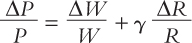
where R denotes the raw material price that must be paid for these imported inputs and γ stands for the importance of intermediate imports in the production of final goods. Combining this markup pricing relationship with a Phillips curve determining wage changes, where the ‘e’ superscript denotes expectations.
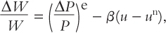
we have
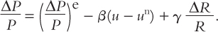
Even when expectations are fully realized, this relationship does not imply that the actual unemployment rate equals the natural rate. Instead, unemployment is given by
Since the price Canadian firms must pay for intermediate imports rises whenever our real exchange rate falls, and since Canada’s real exchange rate was falling significantly through the 1990s, the last term in this equation was positive throughout this period. Thus, the open-economy version of the natural-rate hypothesis implies that Canada’s actual unemployment rate exceeded our natural rate during this period after all.
This reasoning helps makes sense of the American experience in the 1990s as well. Given the closed-economy version of the natural-rate hypothesis, analysts were puzzled as to why U.S. inflation did not accelerate in the late 1990s when the U.S. unemployment rate fell below 4 percent. Many thought that the natural rate was not this low and, with actual and expected inflation likely coinciding at the time, the model predicts rising inflation. But, once again, the last equation directs our attention to the real exchange rate. The Americans’ real exchange rate was rising through the 1990s, and the equation indicates that—with no inflation surprises—the actual unemployment rate must fall below the natural rate. So exchange-rate considerations can go a long way toward answering this challenge to the natural-rate hypothesis.
The second challenge stems from the proposition that the family of short-run Phillips curves may be curves, not straight lines as shown in earlier figures in this chapter. The reason why this might be the case is that wages tend to be less sticky in the upward direction than they are when market pressures are pushing wages down. Statistical studies lend some support to this concern, and Figure 13-6 indicates why this can be important. Figure 13-6 shows two short-run Phillips curves that embody this relative downward rigidity hypothesis in a dramatic way; each Phillips curve is steep when positive inflation is involved and quite flat when negative inflation is involved. One short-run Phillips curve corresponds to underlying expectations of inflation equal to 5 percent, and the other is relevant for zero inflationary expectations.

We compare two long-run situations. First, suppose that the economy has average inflation of 5 percent, but shocks push the economy back and forth between points A and B. Half the time inflation is 6 percent, and the other half of the time inflation is 4 percent. Because the average is 5 percent, it is reasonable to assume inflationary expectations of 5 percent. What are the implications of this volatility for unemployment? Again, because the economy bounces back and forth between points A and B, the average outcome is point C, which corresponds to the natural unemployment rate. Now let us see how things differ when the volatility shifts the outcome between the steep and the flatter regions of a short-run Phillips curve. This occurs in Figure 13-6 if the average inflation rate is zero. In this case, if inflation fluctuates between plus and minus 1 percent, the economy moves between points D and E. Average inflation is zero, but average unemployment is given by the intersection of the straight line joining points D and E and the horizontal axis—that is, by point F. The average unemployment rate exceeds the natural rate.
Thus, as long as the Phillips curve is flatter at low inflation rates and the economy is subject to ongoing shocks, then there is a long-run tradeoff after all—in an average outcomes sense. It appears that we can have lower average unemployment if we choose a small positive inflation rate—enough to make what the evidence shows is a small degree of nonlinearity in the short-run Phillips curves not matter. This is one of the reasons why policymakers often target a low but positive inflation rate instead of zero.
There is one other argument that some economists have stressed to explain why aggregate demand may affect output and employment even in the long run. They have pointed out a number of mechanisms through which recessions might leave permanent scars on the economy by altering the natural rate of unemployment. Hysteresis is the term used to describe the long-lasting influence of history on the natural rate, and hysteresis is the third challenge to the natural-rate hypothesis.
A recession can have permanent effects if it changes the people who become unemployed. For instance, workers might lose valuable job skills when unemployed, lowering their ability to find a job even after the recession ends. Alternatively, a long period of unemployment may change an individual’s attitude toward work and reduce his desire to find employment. In either case, the recession permanently inhibits the process of job search and raises the amount of frictional unemployment.
Another way in which a recession can permanently affect the economy is by changing the process that determines wages. Those who become unemployed may lose their influence on the wage-setting process. Unemployed workers may lose their status as union members, for example. More generally, some of the insiders in the wage-setting process become outsiders. If the smaller group of insiders cares more about high real wages and less about high employment, then the recession may permanently push real wages further above the equilibrium level and raise the amount of wait unemployment.
Hysteresis remains a controversial theory. Some economists believe the theory helps explain persistently high unemployment in Europe, for the rise in European unemployment starting in the early 1980s coincided with disinflation but continued after inflation stabilized. Moreover, the increase in unemployment tended to be larger for those countries that experienced the greatest reductions in inflations, such as Ireland, Italy, and Spain. Yet there is still no consensus whether the hysteresis phenomenon is significant, or why it might be more pronounced in some countries than in others. (Other explanations of high European unemployment, discussed in Chapter 6, give little role to the disinflation.) If true, however, the theory is important, because hysteresis greatly increases the cost of recessions. Put another way, hysteresis raises the sacrifice ratio, because output is lost even after the period of disinflation is over.12