APPENDIX

Components of the Synthesis

493

As explained in this chapter’s conclusion, our dynamic AD–AS model is a simplified version of what is now known as the new neoclassical synthesis. This synthesis is a version of business-cycle theory that blends the microeconomic rigour favoured by classical economists with the recognition of some market failure that is the essence of the Keynesian view. The two approaches that are synthesized are called the new classical and the new Keynesian schools of thought. This Appendix gives you a bit more detail on each of these components of the synthesis.

As a matter of logic, the output of the economy can fluctuate either because the natural level of output fluctuates or because the output of the economy has deviated from its natural level. Throughout most of this book, we have presumed that the natural rate of output grows smoothly over time (as explained by the Solow growth model) and that most short-run fluctuations are deviations from the natural level (as explained by the model of aggregate demand and aggregate supply). New Keynesian theory accepts these presumptions. By contrast, what is known as New Classical theory, or Real Business Cycle theory, suggests that deviations from the natural level are not the whole story and that a significant part of actual fluctuations should be viewed as changes in the natural, or equilibrium, level of output.

According to this theory, short-run economic fluctuations can be explained while maintaining the assumptions of the classical model, which we have used to study the long run. Most important, real business cycle theory assumes that prices are fully flexible, even in the short run. Almost all microeconomic analysis is based on the premise that prices adjust to clear markets. Advocates of real business cycle theory argue that macroeconomic analysis should be based on the same assumption.

Because real business cycle theory assumes complete price flexibility, it is consistent with the classical dichotomy: in this theory, nominal variables, such as the money supply and the price level, do not influence real variables, such as output and employment. To explain fluctuations in real variables, real business cycle theory emphasizes real changes in the economy, such as changes in production technologies, that can alter the economy’s natural level. The “real” in real business cycle theory refers to the theory’s exclusion of nominal variables in explaining short-run economic fluctuations.

By contrast, new Keynesian economics is based on the premise that market-clearing models such as real business cycle theory cannot explain short-run economic fluctuations. In The General Theory, Keynes urged economists to abandon the classical presumption that wages and prices adjust quickly to equilibrate markets. He emphasized that aggregate demand is a primary determinant of national income in the short run. New Keynesian economists accept these basic conclusions, and so they advocate models with sticky wages and prices.

In their research, new Keynesian economists try to develop more fully the Keynesian approach to economic fluctuations. Many new Keynesians accept an extended version of the IS-LM model as their theory of aggregate demand—one that is based on the intertemporal approach to household consumption behaviour that we discuss in Chapter 17 and that has been pioneered by real business cycle theorists. On the supply side, new Keynesians are working to provide a similar theory—an intertemporal-optimization base for the Phillips curve. This work tries to explain how wages and prices behave in the short run by identifying more precisely the market imperfections that make wages and prices sticky and that cause output to deviate from its natural level. We discuss some of this research in the second half of this appendix.

494

In presenting the work of these two schools of thought, this appendix takes an approach that is more descriptive than analytic. Studying recent theoretical developments in detail would require more mathematics than is appropriate for this book. Yet, even without the formal models, we can discuss the direction of this research and get a sense of how different economists are applying micro-economic thinking to better understand macroeconomic fluctuations.⁴

When we studied economic growth in Chapters 7 and 8, we described a relatively smooth process. Output grew as population, capital, and the available technology evolved over time. In the Solow growth model, the economy approaches a steady state in which most variables grow together at a rate determined by the constant rate of technological progress.

But is the process of economic growth necessarily as steady as the Solow model assumes? Perhaps technological progress and economic growth occur unevenly. Perhaps there are shocks to the economy that induce short-run fluctuations in the natural level of output and employment. To see how this might be so, we consider a famous allegory which economists have borrowed from author Daniel Defoe.

Robinson Crusoe is a sailor stranded on a desert island. Because Crusoe lives alone, his life is simple. Yet he has to make many economic decisions. Considering Crusoe’s decisions—and how they change in response to changing circumstances—sheds light on the decisions that people face in larger, more complex economies.

To keep things simple, imagine that Crusoe engages in only a few activities. Crusoe spends some of his time enjoying leisure, perhaps swimming at his island’s beaches. He spends the rest of his time working, either catching fish or collecting vines to make into fishing nets. Both forms of work produce a valuable good: fish are Crusoe’s consumption, and nets are Crusoe’s investment. If we were to compute GDP for Crusoe’s island, we would add together the number of fish caught and the number of nets made (weighted by some “price” to reflect Crusoe’s relative valuation of these two goods).

495

Crusoe allocates his time among swimming, fishing, and making nets based on his preferences and the opportunities available to him. It is reasonable to assume that Crusoe optimizes. That is, he chooses the quantities of leisure, consumption, and investment that are best for him given the constraints that nature imposes.

Over time, Crusoe’s decisions change as shocks impinge on his life. For example, suppose that one day a big school of fish passes by the island. GDP rises in the Crusoe economy for two reasons. First, Crusoe’s productivity rises: with a large school in the water, Crusoe catches more fish per hour of fishing. Second, Crusoe’s employment rises. That is, he decides to reduce temporarily his enjoyment of leisure in order to work harder and take advantage of this unusual opportunity to catch fish. The Crusoe economy is booming.

Similarly, suppose that a storm arrives one day. Because the storm makes outdoor activity difficult, productivity falls: each hour spent fishing or making nets yields a smaller output. In response, Crusoe decides to spend less time working and to wait out the storm in his hut. Consumption of fish and investment in nets both fall, so GDP falls as well. The Crusoe economy is in recession.

Suppose that one day Crusoe is attacked by natives. While he is defending himself, Crusoe has less time to enjoy leisure. Thus, the increased demand for defence spurs employment in the Crusoe economy, especially in the “defence industry.” To some extent, Crusoe spends less time fishing for consumption. To a larger extent, he spends less time making nets, because this task is easy to put off for a while. Thus, defence spending crowds out investment. Because Crusoe spends more time at work, GDP (which now includes the value of national defence) rises. The Crusoe economy is experiencing a wartime boom.

What is notable about this story of booms and recessions is its simplicity. In this story, fluctuations in output, employment, consumption, investment, and productivity are all the natural and desirable response of an individual to the inevitable changes in his environment. In the Crusoe economy, fluctuations have nothing to do with monetary policy, sticky prices, or any type of market failure.

According to the theory of real business cycles, fluctuations in our economy are much the same as fluctuations in Robinson Crusoe’s. Shocks to our ability to produce goods and services (like the changing weather on Crusoe’s island) alter the natural levels of employment and output. These shocks are not necessarily desirable, but they are inevitable. Once the shocks occur, it is desirable for GDP, employment, and other real macroeconomic variables to fluctuate in response.

The parable of Robinson Crusoe, like any model in economics, is not intended to be a literal description of how the economy works. Instead, it tries to get at the essence of the complex phenomenon that we call the business cycle. Does the parable achieve this goal? Are the booms and recessions in modern industrial economies really like the fluctuations on Robinson Crusoe’s island? Economists disagree about the answer to this question and, therefore, disagree about the validity of real business cycle theory. At the heart of the debate are four basic issues:

496

Whether or not you view the parable of Robinson Crusoe as a plausible allegory for the business cycle, considering these four issues is instructive, for each of them raises fundamental questions about how the economy works.

Real business cycle theory emphasizes the idea that the quantity of labour supplied at any given time depends on the incentives that workers face. Just as Robinson Crusoe changes his work effort voluntarily in response to changing circumstances, workers are willing to work more hours when they are well rewarded and are willing to work fewer hours when they are poorly rewarded. Sometimes, if the reward for working is sufficiently small, workers choose to forgo working altogether—at least temporarily. This willingness to reallocate hours of work over time is called the intertemporal substitution of labour.

To see how intertemporal substitution affects labour supply, consider the following example. A university student finishing her second year has two summer vacations left before graduation. She wishes to work for one of these summers (so she can buy a car after she graduates) and to relax at the beach during the other summer. How should she choose which summer to work?

Let W₁ be her real wage in the first summer and W₂ the real wage she expects in the second summer. To choose which summer to work, the student compares these two wages. Yet, because she can earn interest on money earned earlier, a dollar earned in the first summer is more valuable than a dollar earned in the second summer. Let r be the real interest rate. If the student works in the first summer and saves her earnings, she will have (1 + r)W₁ a year later. If she works in the second summer, she will have W₂. The intertemporal relative wage—that is, the earnings from working the first summer relative to the earnings from working the second summer—is

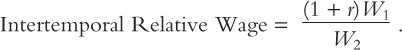
Working the first summer is more attractive if the interest rate is high or if the wage is high relative to the wage expected to prevail in the future.

497

According to real business cycle theory, all workers perform this cost–benefit analysis when deciding whether to work or to enjoy leisure. If the wage is temporarily high or if the interest rate is high, it is a good time to work. If the wage is temporarily low or if the interest rate is low, it is a good time to enjoy leisure.

Real business cycle theory uses the intertemporal substitution of labour to explain why employment and output fluctuate. Shocks to the economy that cause the interest rate to rise or the wage to be temporarily high cause people to want to work more. The increase in work effort raises employment and production. Shocks that cause the interest rate to fall or the wage to be temporarily low decrease employment and production.

Critics of real business cycle theory believe that fluctuations in employment do not reflect changes in the amount people want to work. They believe that desired employment is not very sensitive to the real wage and the real interest rate. They point out that the unemployment rate fluctuates substantially over the business cycle. The high unemployment in recessions suggests that the labour market does not clear: if people were voluntarily choosing not to work in recessions, they would not call themselves unemployed. These critics conclude that wages do not adjust to equilibrate labour supply and labour demand, as real business cycle models assume.

In reply, advocates of real business cycle theory argue that unemployment statistics are difficult to interpret. The mere fact that the unemployment rate is high does not mean that intertemporal substitution of labour is unimportant. Individuals who voluntarily choose not to work may call themselves unemployed so they can collect employment-insurance benefits. Or they may call themselves unemployed because they would be willing to work if they were offered the wage they receive in most years.

The Crusoe economy fluctuates because of changes in the weather, which induce Crusoe to alter his work effort. In real business cycle theory, the analogous variable is technology, which determines an economy’s ability to turn inputs (capital and labour) into output (goods and services). The theory assumes that our economy experiences fluctuations in technology and that these fluctuations in technology, that are called technology shocks, cause fluctuations in output and employment. When the available production technology improves, the economy produces more output, and real wages rise. Because of intertemporal substitution of labour, the improved technology also leads to greater employment. Real business cycle theorists often explain recessions as periods of “technological regress.” According to these models, output and employment fall during recessions because the available production technology deteriorates, lowering output and reducing the incentive to work.

Critics of real business cycle theory are skeptical that the economy experiences large shocks to technology. It is a more common presumption that technological progress occurs gradually. Critics argue that technological regress is especially implausible: the accumulation of technological knowledge may slow down, but it is hard to imagine that it would go in reverse.

498

Advocates respond by taking a broad view of shocks to technology. They argue that there are many events that, although not literally technological, affect the economy much as technology shocks do. For example, bad weather, the passage of strict environmental regulations, or increases in raw material prices have effects similar to adverse changes in technology: they all reduce our ability to turn capital and labour into goods and services. Whether such events are sufficiently common to explain the frequency and magnitude of business cycles is an open question.

Just as money has no role in the Crusoe economy, real business cycle theory assumes that money in our economy is neutral, even in the short run. That is, monetary policy is assumed not to affect real variables such as output and employment. Not only does the neutrality of money give real business cycle theory its name, but neutrality is also the theory’s most radical assumption.

Critics argue that the evidence does not support short-run monetary neutrality. They point out that reductions in money growth and inflation are almost always associated with periods of high unemployment. Monetary policy appears to have a strong influence on the real economy.

Advocates of real business cycle theory argue that their critics confuse the direction of causation between money and output. These advocates claim that the money supply is endogenous: fluctuations in output might cause fluctuations in the money supply. For example, when output rises because of a beneficial technology shock, the quantity of money demanded rises. The Bank of Canada may respond by raising the money supply to accommodate the greater demand. This endogenous response of money to economic activity may give the illusion of monetary non-neutrality.⁵

Real business cycle theory assumes that wages and prices adjust quickly to clear markets, just as Crusoe always achieves his optimal level of GDP without any impediment from a market imperfection. Advocates of this theory believe that the market imperfection of sticky wages and prices is not important for understanding economic fluctuations. They also believe that the assumption of flexible prices is superior methodologically to the assumption of sticky prices, because it ties macroeconomic theory more closely to microeconomic theory.

500

Critics point out that many wages and prices are not flexible. They believe that this inflexibility explains both the existence of unemployment and the non-neutrality of money. To explain why prices are sticky, they rely on the various new Keynesian theories that we discuss in the next section.⁸

Most economists are skeptical of the basic version of the theory of real business cycles and believe that short-run fluctuations in output and employment involve deviations from the economy’s natural levels of these variables. They think these deviations occur because wages and prices are slow to adjust to changing economic conditions. As we have discussed in Chapters 9, 13, and earlier in the present chapter, this stickiness makes the short-run aggregate supply curve upward sloping rather than vertical. As a result, fluctuations in aggregate demand cause short-run fluctuations in output and employment. The most recent generation of real business cycle models have embraced the hypothesis of sticky prices, so that both demand and technology shocks play a role in determining cycles. As a result, as noted already, a synthesis has developed in modern research in macroeconomics.⁹

But why exactly are prices sticky? New Keynesian research has attempted to answer this question by examining the microeconomics behind short-run price adjustment. By doing so, it tries to put the traditional theories of short-run fluctuations on a firmer theoretical foundation.

One reason prices do not adjust immediately in the short run is that there are costs to price adjustment. To change its prices, a firm may need to send out a new catalogue to customers, distribute new price lists to its sales staff, or, in the case of a restaurant, print new menus. These costs of price adjustment, called menu costs, lead firms to adjust prices intermittently rather than continuously.

501

Economists disagree about whether menu costs explain the short-run stickiness of prices. Skeptics point out that menu costs are usually very small. How can small menu costs help to explain recessions, which are very costly for society? Proponents reply that small does not mean inconsequential: even though menu costs are small for the individual firm, they can have large effects on the economy as a whole.

According to proponents of the menu-cost hypothesis, to understand why prices adjust slowly, we must acknowledge that there are externalities to price adjustment: a price reduction by one firm benefits other firms in the economy. When a firm lowers the price it charges, it slightly lowers the average price level and thereby raises real money balances. The increase in real money balances expands aggregate income (by shifting the LM curve outward). The economic expansion in turn raises the demand for the products of all firms. This macro-economic impact of one firm’s price adjustment on the demand for all other firms’ products is called an aggregate-demand externality.

In the presence of this aggregate-demand externality, small menu costs can make prices sticky, and this stickiness can have a large cost to society. Suppose that a firm originally sets its price too high and later must decide whether to cut its price. The firm makes this decision by comparing the benefit of a price cut—higher sales and profit—to the cost of price adjustment. Yet because of the aggregate-demand externality, the benefit to society of the price cut would exceed the benefit to the firm. The firm ignores this externality when making its decision, so it may decide not to pay the menu cost and cut its price even though the price cut is socially desirable. Hence, sticky prices may be optimal for those setting prices, even though they are undesirable for the economy as a whole.¹⁰

Some new Keynesian economists suggest that recessions result from a failure of coordination among economic decisionmakers. In recessions, output is low, workers are unemployed, and factories sit idle. It is possible to imagine allocations of resources in which everyone is better off—for example, the high output and employment of the 1920s were clearly preferable to the low output and employment of the 1930s. If society fails to reach an outcome that is feasible and that everyone prefers, then the members of society have failed to coordinate their behaviour in some way.

Coordination problems can arise in the setting of wages and prices because those who set them must anticipate the actions of other wage and price setters. Union leaders negotiating wages are concerned about the concessions other unions will win. Firms setting prices are mindful of the prices other firms will charge.

To see how a recession could arise as a failure of coordination, consider the following parable. The economy is made up of two firms. After a fall in the money supply, each firm must decide whether to cut its price, based on its goal of maximizing profit. Each firm’s profit, however, depends not only on its pricing decision but also on the decision made by the other firm.

503

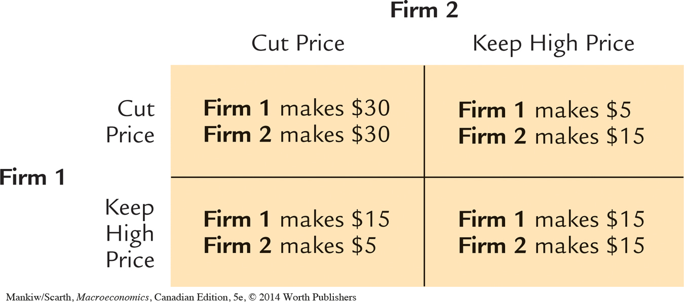
The choices facing each firm are listed in Table 14-2, which shows how the profits of the two firms depend on their actions. If neither firm cuts its price, real money balances are low, a recession ensues, and each firm makes a profit of only $15. If both firms cut their prices, real money balances are high, a recession is avoided, and each firm makes a profit of $30. Although both firms prefer to avoid a recession, neither can do so by its own actions. If one firm cuts its price while the other does not, a mild recession follows. The firm making the price cut gains customers but gets less revenue from each one. If demand is inelastic, the price-cutting firm will lose; in the example depicted in Table 14-2, this firm makes only $5, while the other firm makes $15.

The essence of this parable is that each firm’s decision influences the set of outcomes available to the other firm. When one firm cuts its price, it improves the position of the other firm, because the other firm can then act to avoid the recession. This positive impact of one firm’s price cut on the other firm’s profit opportunities might arise from an aggregate-demand externality.

What outcome should we expect in this economy? On the one hand, if each firm expects the other to cut its price, both will cut prices, resulting in the preferred outcome in which each makes $30. On the other hand, if each firm expects the other to maintain its price, both will maintain their prices, resulting in the inferior result in which each makes $15. Either of these outcomes is possible: economists say that there are multiple equilibria.

The inferior outcome, in which each firm makes $15, is an example of a coordination failure. If the two firms could coordinate, they would both cut their price and reach the preferred outcome. In the real world, unlike in our parable, coordination is often difficult because the number of firms setting prices is large. The moral of the story is that prices can be sticky simply because people expect them to be sticky, even though stickiness is in no one’s interest.¹²

504

Not everyone in the economy sets new wages and prices at the same time. Instead, the adjustment of wages and prices throughout the economy is staggered. Staggering slows the process of coordination and price adjustment. In particular, staggering makes the overall level of wages and prices adjust gradually, even when individual wages and prices change frequently.

Consider the following example, which, for simplicity, involves no aggregate-demand externality. Suppose first that price setting is synchronized: every firm adjusts its price on the first day of every month. If the money supply and aggregate demand rise on May 10, output will be higher from May 10 to June 1 because prices are fixed during this interval. But on June 1 all firms will raise their prices in response to the higher demand, ending the boom.

505

Now suppose that price setting is staggered: half the firms set prices on the first of each month and half on the fifteenth. If the money supply rises on May 10, then half the firms can raise their prices on May 15. But if the demand for their product is elastic, these firms will probably not raise their prices very much. Because half the firms will not be changing their prices on the fifteenth, a price increase by any firm will raise that firm’s relative price, causing it to lose customers. (By contrast, if all firms are synchronized, all firms can raise prices together, leaving relative prices unaffected.) If the May 15 price setters make little adjustment in their prices, then the other firms will make little adjustment when their turn comes on June 1, because they also want to avoid relative price changes. And so on. The price level rises slowly as the result of small price increases on the first and the fifteenth of each month. Hence, staggering makes the overall price level adjust sluggishly, because no firm wishes to be the first to post a substantial price increase.

Staggering also affects wage determination. Consider, for example, how a fall in the money supply works its way through the economy. A smaller money supply reduces aggregate demand, which in turn requires a proportionate fall in nominal wages to maintain full employment. Each worker might be willing to take a lower nominal wage if all other wages were to fall proportionately. The worker could then reasonably expect a reduction in the overall level of goods prices. But each worker is reluctant to be the first to take a pay cut, knowing that this means, at least temporarily, a fall in his or her relative wage. Since the setting of wages is staggered, the reluctance of each worker to reduce his or her wage first makes the overall level of wages slow to respond to changes in aggregate demand. In other words, the staggered setting of individual wages makes the overall level of wages sticky.¹⁴

Recent developments in the theory of short-run economic fluctuations remind us that we do not understand economic fluctuations as well as we would like. Fundamental questions about the economy remain open to dispute. Is the stickiness of wages and prices a key to understanding economic fluctuations? Does monetary policy have real effects?

The way economists answer these questions affects how they view the role of economic policy. Economists who believe that wages and prices are sticky, such as those pursuing new Keynesian theories, often believe that monetary and fiscal policy should be used to try to stabilize the economy. Price stickiness is a type of market imperfection, and so it is possible, but not necessarily the case that stabilization policies can raise economic well-being for society as a whole.

506

By contrast, the basic version of the real business cycle theory suggests that the government’s influence on the economy is limited and that even if the government could stabilize the economy, it should not try to do so. According to this theory, the ups and downs of the business cycle are the natural and efficient response of the economy to changing technological possibilities. The standard real business cycle model does not include any type of market imperfection. In this model, the “invisible hand” of the marketplace guides the economy to an optimal allocation of resources.

Although this appendix has divided recent research into two distinct camps, not all economists fall entirely into one camp or the other. Over time, more economists have been trying to incorporate the strengths of both approaches into their research. Real business cycle theory places a heavy emphasis on intertemporal optimization and forward-looking behaviour, while new Keynesian theory stresses the importance of sticky prices and other market imperfections. Increasingly, theories at the research frontier meld many of these elements to advance our understanding of economic fluctuations. It is this kind of work that makes macroeconomics an exciting field of study.¹⁵

New Keynesian economics

Real business cycle theory

Intertemporal substitution of labour

Technology shocks

Menu costs

Aggregate-demand externality

Coordination failure