Chapter 21. Evolution: How Genotypes and Phenotypes Change over Time

Early population geneticists relied on observable traits and gel electrophoresis to measure variation.

It would be a simple matter to measure genetic variation in a population if we could use observable traits. Then we could simply count the individuals displaying variant forms of a trait and have a measure of the variation of that trait’s gene. However, as we saw in Chapter 18, this approach can work only rarely, for two important reasons. First, many traits are encoded by a large number of genes. In these cases, it is difficult, if not impossible, to make direct inferences from a phenotype to the underlying genotype. Even traits that seem to have a simple set of phenotypes often prove to have a complicated genetic basis. For instance, human skin color is determined by at least six different genes. Second, the phenotype is a product of both the genotype and the environment.

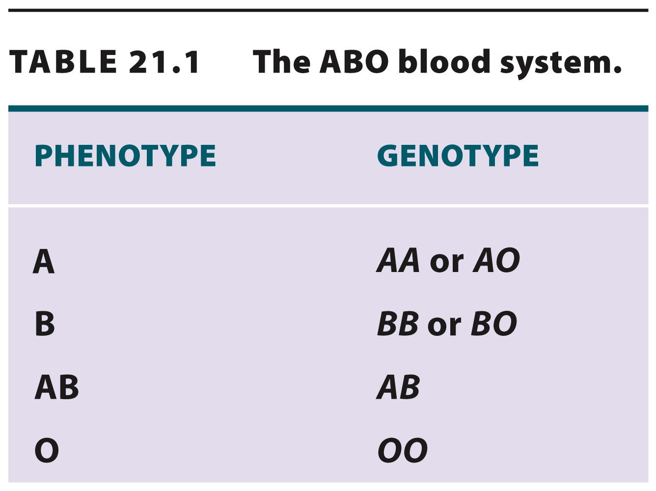
FIG. 21.3 Single-gene variation. A genetic difference in color in the two-spot ladybug, Adalia bipunctata, results from variation in a single gene.

Until the 1960s, there was only one workable solution: to limit population genetics to the study of phenotypes that are encoded by a single gene. As these are few, the number of genes that population geneticists could study was extremely small. Human blood groups, including the ABO system, provided an early example of a trait encoded by a single gene with multiple alleles. 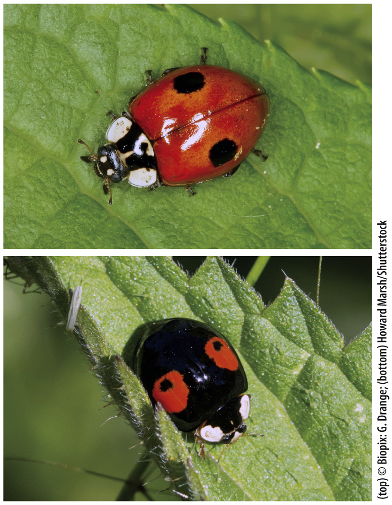At this gene, there are three alleles in the population—A, B, and O—and therefore six possible genotypes, which result in four different phenotypes (Table 21.1).

Other instances in which phenotypic variation can be readily correlated with genotype include certain markings in invertebrates. For example, the coloring of the two-spot ladybug Adalia bipunctata is controlled by a single gene (Fig. 21.3). However, the genetic basis of most traits is not so simple.

Single-gene variation became much easier to detect in the 1960s with the application of gel electrophoresis. In Chapter 12, we saw how gel electrophoresis separates segments of DNA according to their size. Before DNA technologies were developed, the same basic process was applied to proteins to separate them according to their electrical charge and their size. In gel electrophoresis, the proteins being studied migrate through a gel when an electrical charge is applied. The rate at which the proteins move from one end of the gel to the other is determined by their charge and their size.

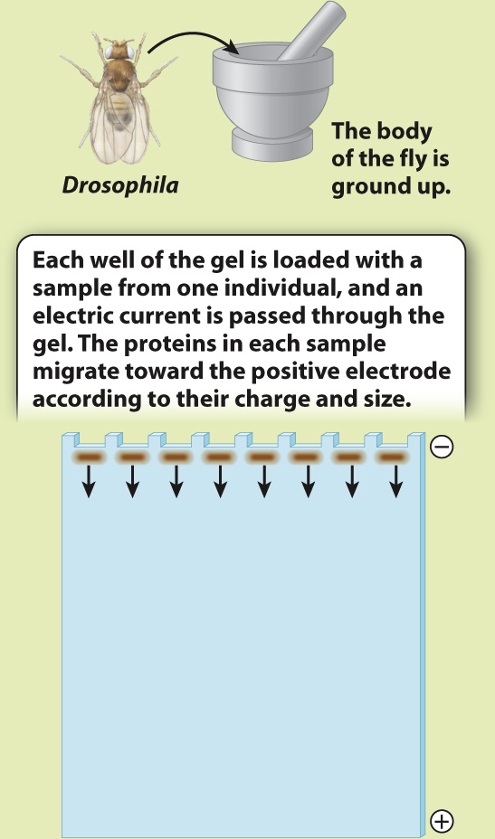
Early studies of protein electrophoresis focused on enzymes that catalyze reactions that can be induced to produce a dye when the substrate for the enzyme is added. If we add the substrate, we can see the locations of the proteins in the gel. The bands in the gel provide a visual picture of genetic variation in the population, revealing what alleles are present and what their frequencies are. Fig. 21.4 shows this sort of experiment.

HOW DO WE KNOW?

FIG. 21.4

How is genetic variation measured?

BACKGROUND The introduction of protein gel electrophoresis in 1966 gave researchers the opportunity to identify differences in amino acid sequence in proteins both among individuals and, in the case of heterozygotes, within individuals. Proteins with different amino acid sequences run at different rates through a gel in an electric field. Often, a single amino acid difference is enough to affect the mobility of a protein in a gel.

METHOD Starting with crude tissue—in this case, the ground-up whole body of a fruit fly—we load the material on a gel and turn on the current. The rate at which a protein migrates depends on its size and charge, both of which may be affected by its amino acid sequence. To visualize the protein at the end of the gel run, we use a biochemical indicator that produces a stain when the protein of interest is active. Here, we use an indicator that detects the activity of alcohol dehydrogenase (Adh). The result is a series of bands on the gel showing where the Adh proteins in each lane migrated.

RESULTS The Adh gene has two common alleles, distinguished by a single amino acid difference that changes the charge of the protein. One allele, Fast (F), accordingly runs faster than the other, Slow (S). Four individuals are S homozygotes; two are F homozygotes; and two are FS heterozygotes. Note that the heterozygotes do not stain as strongly on the gel because each band has half the intensity of the single band in the homozygote. We can measure the allele frequencies simply by counting the alleles. Each homozygote has two of the same allele, and each heterozygote has one of each.

FIG. 21.4

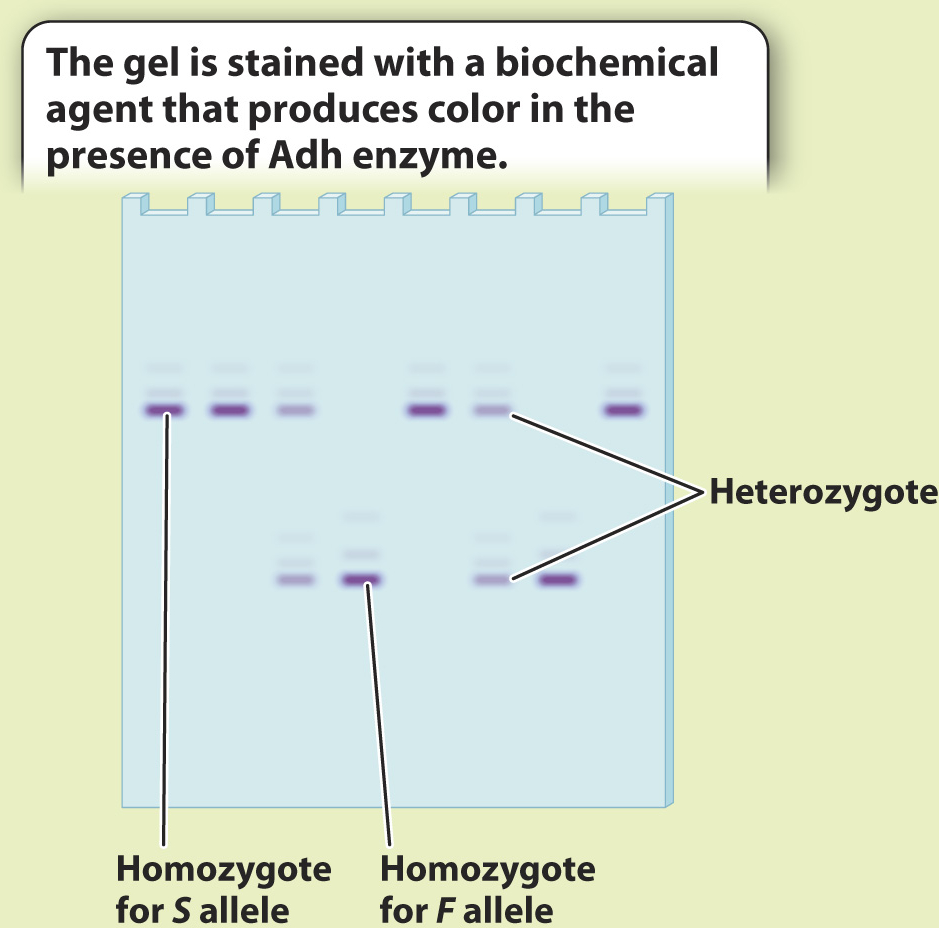
Total number of alleles in the population of 8 individuals = 8 × 2 = 16

Number of S in the population = 2 × (number of S homozygotes) + (number of heterozygotes) = 8 + 2 = 10

Frequency of

Number of F in the population = 2 × (number of F homozygotes) + (number of heterozygotes) = 4 + 2 = 6

Frequency of

Note that the two allele frequencies add to 1.

CONCLUSION We now have a profile of genetic variation at this gene for these individuals. Population genetics involves comparing data such as these with data collected from other populations to determine the forces shaping patterns of genetic variation.

FOLLOW-UP WORK This technique is seldom used these days because it is easy now to recover much more detailed genetic information about genetic variation from DNA sequencing.

SOURCE Lewontin, R. C., and J. L. Hubby. 1966. “A Molecular Approach to the Study of Genic Heterozygosity in Natural Populations. II. Amount of Variation and Degree of Heterozygosity in Natural Populations of Drosophila pseudoobscura.” Genetics 54:595–609.