In 1958, American chemist Charles David Keeling began a novel program to monitor the atmosphere. At the time he began his study, scientists had only a vague notion of how carbon dioxide (CO₂) behaves in air. Many thought that CO₂ might vary unpredictably from time to time, and from place to place. Keeling decided to find out if in fact it did. From five towers set high on Mauna Loa in Hawaii, 3400 m above sea level, he sampled the atmosphere every hour and measured its composition with an infrared gas analyzer. Within the first few years of his project, a pattern of seasonal oscillation became apparent: CO₂ concentration in the air reached its annual high point in spring and then declined by about 6 parts per million (ppm, by volume) to a minimum in early fall (Fig. 25.1). Such regular variation was unexpected: What could be causing it?

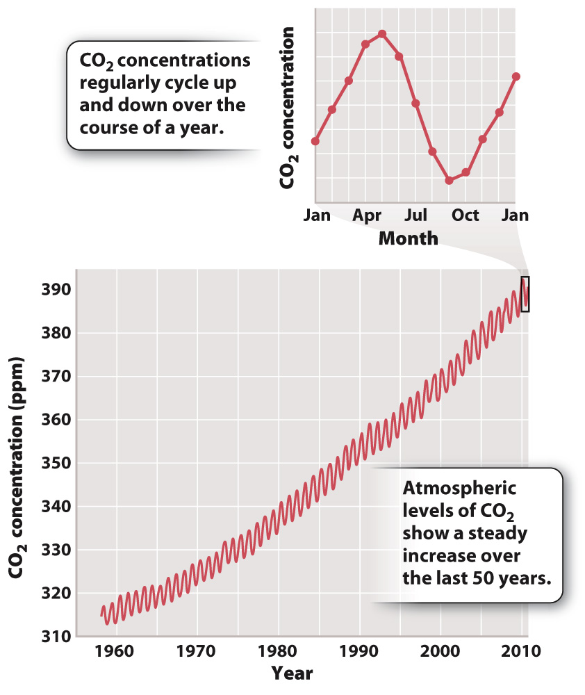
Perhaps the pattern was local. Airplane traffic to Hawaii peaked in winter, and maybe that was affecting the air around Mauna Loa. As measurements continued through a number of years, however, the pattern persisted, even as trends in air traffic changed. Moreover, monitoring stations in many other parts of the globe gave similar results. Knowing that the Mauna Loa measurements are representative of the atmosphere as a whole allows us to appreciate what an annual variation of 6 ppm really means. With calendar-like regularity, approximately 47 billion metric tons of CO₂ were entering and leaving the atmosphere annually—that’s 13 billion metric tons of the element carbon (the rest of the mass is oxygen). To explain such a pattern, we must consider processes that affect the planet as a whole.

A second pattern is evident in Fig. 25.1. Summertime removal of CO₂ from the atmosphere does not quite balance winter increase, with the result that the amount of CO₂ in the atmosphere on any given date is greater than it was a year earlier. Atmospheric CO₂ levels have therefore increased steadily through the period of monitoring. For example, mean annual CO₂ levels, about 315 ppm in 1958, reached 404 ppm by late April 2015. This is an increase of more than 25%, and there is no indication that the rise will slow or stop any time soon.

What causes atmospheric CO₂ to vary through the year and over a timescale of decades? To answer this question, we need to ask what processes introduce CO₂ into the atmosphere and what processes remove it. Carbon dioxide is added to the atmosphere by (1) geologic inputs, mainly from volcanoes and mid-ocean ridges; (2) biological inputs, especially respiration; and (3) human activities, including deforestation and the burning of fossil fuels. Processes that remove CO₂ from the atmosphere include (1) geologic removal, especially by chemical weathering in which CO₂ in rainwater reacts with exposed rocks, and (2) biological removal, mainly through photosynthesis. As we will see, geologic processes play key roles in the carbon cycle on timescales of centuries and longer. Only biology, however, can account for the annual rhythm of the Keeling curve.

511