1.3 Statistical Reasoning in Everyday Life
Asked about the ideal wealth distribution in America, Democrats and Republicans were surprisingly similar. In the Democrats’ ideal world, the richest 20 percent would possess 30 percent of the wealth. Republicans preferred a similar 35 percent (Norton & Ariely, 2011).
43
In descriptive, correlational, and experimental research, statistics are tools that help us see and interpret what the unaided eye might miss. Sometimes the unaided eye misses badly. Researchers Michael Norton and Dan Ariely (2011) invited 5522 Americans to estimate the percent of wealth possessed by the richest 20 percent in their country. The average person’s guess—
When setting goals, we love big round numbers. We’re far more likely to want to lose 20 pounds than 19 or 21 pounds. We’re far more likely to retake the SAT if our verbal plus math score is just short of a big round number, such as 1200. By modifying their behavior, batters are nearly four times more likely to finish the season with a .300 average than with a .299 average (Pope & Simonsohn, 2011).
Accurate statistical understanding benefits everyone. To be an educated person today is to be able to apply simple statistical principles to everyday reasoning. One needn’t memorize complicated formulas to think more clearly and critically about data.

Off-
- Ten percent of people are homosexual. Or is it 2 to 4 percent, as suggested by various national surveys (Chapter 11)?
- We ordinarily use only 10 percent of our brain. Or is it closer to 100 percent (Chapter 2)?
- The human brain has 100 billion nerve cells. Or is it more like 40 billion, as suggested by extrapolation from sample counts (Chapter 2)?
The point to remember: Doubt big, round, undocumented numbers. That’s actually a lesson we intuitively appreciate, by finding precise numbers more credible (Oppenheimer et al., 2014). When U.S. Secretary of State John Kerry sought to rally American support in 2013 for a military response to Syria’s apparent use of chemical weapons, his argument gained credibility from its precision: “The United States government now knows that at least 1429 Syrians were killed in this attack, including at least 426 children.”
Statistical illiteracy also feeds needless health scares (Gigerenzer et al., 2008, 2009, 2010). In the 1990s, the British press reported a study showing that women taking a particular contraceptive pill had a 100 percent increased risk of blood clots that could produce strokes. This caused thousands of women to stop taking the pill, leading to a wave of unwanted pregnancies and an estimated 13,000 additional abortions (which also are associated with increased blood-
Describing Data
1-
Once researchers have gathered their data, they may use descriptive statistics to organize that data meaningfully. One way to do this is to convert the data into a simple bar graph, as in FIGURE 1.8 below, which displays a distribution of different brands of trucks still on the road after a decade. When reading statistical graphs such as this, take care. It’s easy to design a graph to make a difference look big (Figure 1.8a) or small (Figure 1.8b). The secret lies in how you label the vertical scale (the y-
The point to remember: Think smart. When viewing graphs, read the scale labels and note their range.
RETRIEVAL PRACTICE

Read the scale labels
- An American truck manufacturer offered graph (a)—with actual brand names included—to suggest the much greater durability of its trucks. What does graph (b) make clear about the varying durability, and how is this accomplished?
Note how the y-axis of each graph is labeled. The range for the y-axis label in graph (a) is only from 95 to 100. The range for graph (b) is from 0 to 100. All the trucks rank as 95% and up, so almost all are still functioning after 10 years, which graph (b) makes clear.
Measures of Central Tendency
mode the most frequently occurring score(s) in a distribution.
The next step is to summarize the data using some measure of central tendency, a single score that represents a whole set of scores. The simplest measure is the mode, the most frequently occurring score or scores. The most familiar is the mean, or arithmetic average—
mean the arithmetic average of a distribution, obtained by adding the scores and then dividing by the number of scores.
median the middle score in a distribution; half the scores are above it and half are below it.
Measures of central tendency neatly summarize data. But consider what happens to the mean when a distribution is lopsided, when it’s skewed by a few way-
The average person has one ovary and one testicle.
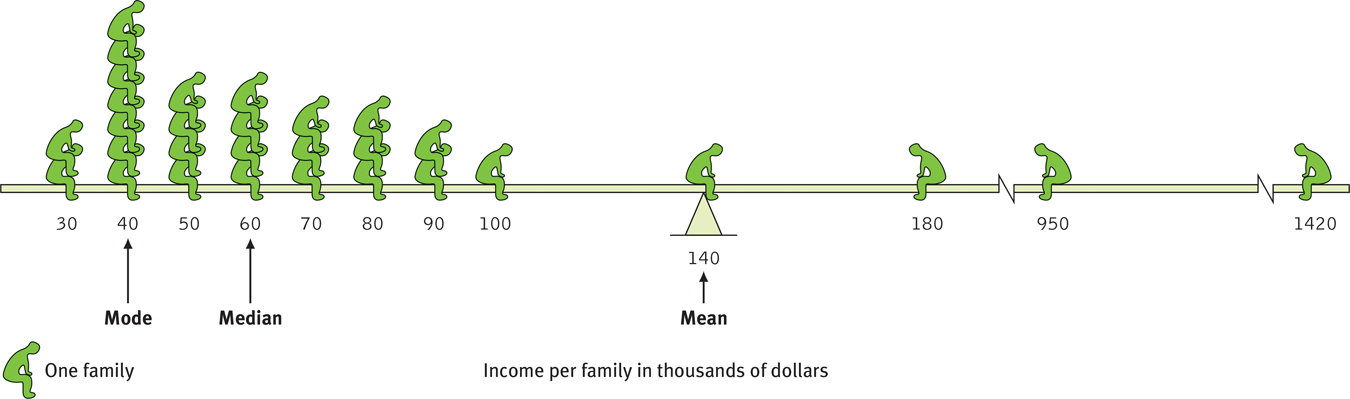
A skewed distribution This graphic representation of the distribution of a village’s incomes illustrates the three measures of central tendency—
44
The point to remember: Always note which measure of central tendency is reported. If it is a mean, consider whether a few atypical scores could be distorting it.
Measures of Variation
Knowing the value of an appropriate measure of central tendency can tell us a great deal. But the single number omits other information. It helps to know something about the amount of variation in the data—
45
range the difference between the highest and lowest scores in a distribution.
The range of scores—
The more useful standard for measuring how much scores deviate from one another is the standard deviation. It better gauges whether scores are packed together or dispersed, because it uses information from each score. The computation (see TABLE 1.4 for an example) assembles information about how much individual scores differ from the mean. If your college or university attracts students of a certain ability level, their intelligence scores will have a relatively small standard deviation compared with the more diverse community population outside your school.

Standard Deviation Is Much More Informative Than Mean Alone
Note that the test scores in Class A and Class B have the same mean (80), but very different standard deviations, which tell us more about how the students in each class are really faring.
standard deviation a computed measure of how much scores vary around the mean score.
normal curve (normal distribution) a symmetrical, bell-shaped curve that describes the distribution of many types of data; most scores fall near the mean (about 68 percent fall within one standard deviation of it) and fewer and fewer near the extremes.
You can grasp the meaning of the standard deviation if you consider how scores tend to be distributed in nature. Large numbers of data—
As FIGURE 1.10 shows, a useful property of the normal curve is that roughly 68 percent of the cases fall within one standard deviation on either side of the mean. About 95 percent of cases fall within two standard deviations. Thus, as Chapter 10 notes, about 68 percent of people taking an intelligence test will score within ±15 points of 100. About 95 percent will score within ±30 points.
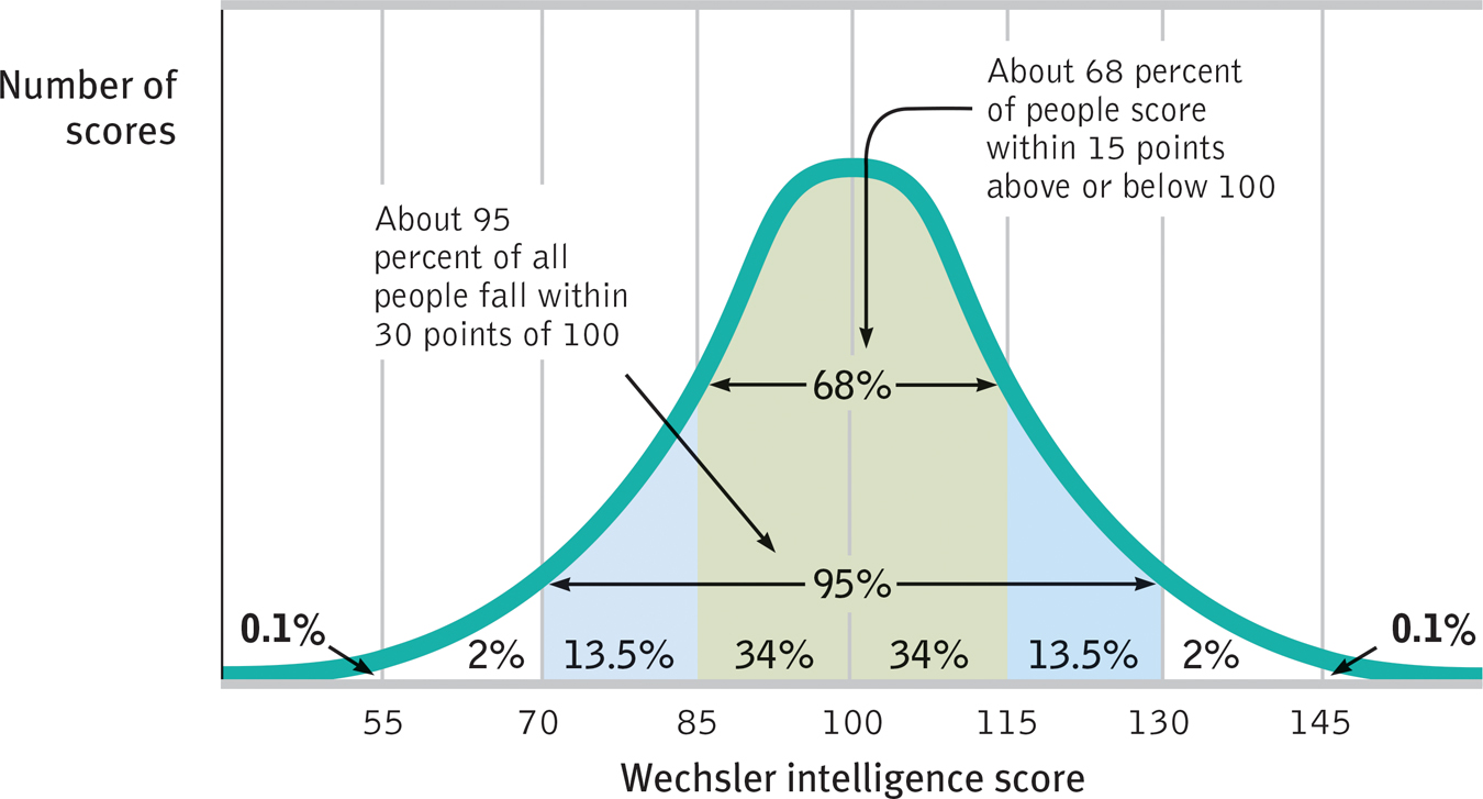
The normal curve Scores on aptitude tests tend to form a normal, or bell-
46
 For an interactive tutorial on these statistical concepts, visit LaunchPad’s PsychSim 6: Descriptive Statistics.
RETRIEVAL PRACTICE
- The average of a distribution of scores is the ______________. The score that shows up most often is the ______________. The score right in the middle of a distribution (half the scores above it; half below) is the ______________. We determine how much scores vary around the average in a way that includes information about the ______________ of scores (difference between highest and lowest) by using the ______________ ______________ formula.
mean; mode; median; range; standard deviation
Significant Differences
1-
Data are “noisy.” The average score in one group (children who were breast-
When Is an Observed Difference Reliable?
In deciding when it is safe to generalize from a sample, we should keep three principles in mind:
- Representative samples are better than biased samples. The best basis for generalizing is not from the exceptional and memorable cases one finds at the extremes but from a representative sample of cases. Research never randomly samples the whole human population. Thus, it pays to keep in mind what population a study has sampled.
- Less-variable observations are more reliable than those that are more variable. As we noted earlier in the example of the basketball player whose game-to-game points were consistent, an average is more reliable when it comes from scores with low variability.
- More cases are better than fewer. An eager prospective student visits two university campuses, each for a day. At the first, the student randomly attends two classes and discovers both instructors to be witty and engaging. At the next campus, the two sampled instructors seem dull and uninspiring. Returning home, the student (discounting the small sample size of only two teachers at each institution) tells friends about the “great teachers” at the first school, and the “bores” at the second. Again, we know it but we ignore it: Averages based on many cases are more reliable (less variable) than averages based on only a few cases.
The point to remember: Smart thinkers are not overly impressed by a few anecdotes. Generalizations based on a few unrepresentative cases are unreliable.
47
When Is an Observed Difference Significant?
Perhaps you’ve compared men’s and women’s scores on a laboratory test of aggression, and found a gender difference. But individuals differ. How likely is it that the difference you observed was just a fluke? Statistical testing can estimate that.
Here is the underlying logic: When averages from two samples are each reliable measures of their respective populations (as when each is based on many observations that have small variability), then their difference is likely to be reliable as well. (Example: The less the variability in women’s and in men’s aggression scores, the more confidence we would have that any observed gender difference is reliable.) And when the difference between the sample averages is large, we have even more confidence that the difference between them reflects a real difference in their populations.

statistical significance a statistical statement of how likely it is that an obtained result occurred by chance.
In short, when sample averages are reliable, and when the difference between them is relatively large, we say the difference has statistical significance. This means that the observed difference is probably not due to chance variation between the samples.

For a 9.5-minute video synopsis of psychology’s scientific research strategies, visit LaunchPad’s Video: Research Methods.
In judging statistical significance, psychologists are conservative. They are like juries who must presume innocence until guilt is proven. For most psychologists, proof beyond a reasonable doubt means not making much of a finding unless the odds of its occurring by chance, if no real effect exists, are less than 5 percent.
When reading about research, you should remember that, given large enough or homogeneous enough samples, a difference between them may be “statistically significant” yet have little practical significance. For example, comparisons of intelligence test scores among hundreds of thousands of first-
The point to remember: Statistical significance indicates the likelihood that a result will happen by chance. But this does not say anything about the importance of the result.
RETRIEVAL PRACTICE
- Can you solve this puzzle?
The registrar’s office at the University of Michigan has found that usually about 100 students in Arts and Sciences have perfect marks at the end of their first term at the University. However, only about 10 to 15 students graduate with perfect marks. What do you think is the most likely explanation for the fact that there are more perfect marks after one term than at graduation (Jepson et al., 1983)?
Averages based on fewer courses are more variable, which guarantees a greater number of extremely low and high marks at the end of the first term.
- ______________ statistics summarize data, while ______________ statistics determine if data can be generalized to other populations.
Descriptive; inferential
48
REVIEW: Statistical Reasoning in Everyday Life

|
REVIEW | Statistical Reasoning in Everyday Life |
LEARNING OBJECTIVES
RETRIEVAL PRACTICE Take a moment to answer each of these Learning Objective Questions (repeated here from within this section). Then click the 'show answer' button to check your answers. Research suggests that trying to answer these questions on your own will improve your long-
1-
measure of central tendency is a single score that represents a whole set of scores. Three such measures that we use to describe data are the mode (the most frequently occurring score), the mean (the arithmetic average), and the median (the middle score in a group of data).
Measures of variation tell us how diverse data are. Two measures of variation are the range (which describes the gap between the highest and lowest scores) and the standard deviation (which states how much scores vary around the mean, or average, score). Scores often form a normal (or bell-shaped) curve.
1-
To feel confident about generalizing an observed difference to other populations, we would want to know that the sample studied was representative of the larger population being studied; that the observations, on average, had low variability; that the sample consisted of more than a few cases; and that the observed difference was statistically significant.
TERMS AND CONCEPTS TO REMEMBER
RETRIEVAL PRACTICE Match each of the terms on the left with its definition on the right. Click on the term first and then click on the matching definition. As you match them correctly they will move to the bottom of the activity.
Question
mode mean median range standard deviation normal curve statistical significance | the arithmetic average of a distribution, obtained by adding the scores and then dividing by the number of scores. a computed measure of how much scores vary around the mean score. the difference between the highest and lowest scores in a distribution. the middle score in a distribution; half the scores are above it and half are below it. (normal distribution) a symmetrical, bell-shaped curve that describes the distribution of many types of data; most scores fall near the mean (about 68 percent fall within one standard deviation of it) and fewer and fewer near the extremes. the most frequently occurring score(s) in a distribution. a statistical statement of how likely it is that an obtained result occurred by chance. |
Use  to create your personalized study plan, which will direct you to the resources that will help you most in
.
to create your personalized study plan, which will direct you to the resources that will help you most in
.
TEST
YOUR-
SELF THINKING CRITICALLY WITH PSYCHOLOGICAL SCIENCE
Test yourself repeatedly throughout your studies. This will not only help you figure out what you know and don’t know; the testing itself will help you learn and remember the information more effectively thanks to the testing effect.
 The Need for Psychological Science
Question
1. refers to our tendency to perceive events as obvious or inevitable after the fact.
Question
2. As scientists, psychologists
| A. |
| B. |
| C. |
| D. |
Question
3. How can critical thinking help you evaluate claims in the media, even if you’re not a scientific expert on the issue?
Critical thinking examines assumptions, appraises the source, discerns hidden values, evaluates evidence, and assesses conclusions. In evaluating a claim in the media, look for any signs of empirical evidence, preferably from several studies. Ask the following questions in your analysis: Are claims based on scientific findings? Have several studies replicated the findings and confirmed them? Are any experts cited? If so, research their background. Are they affiliated with a credible university, college, or institution? Have they conducted or written about scientific research?
Research Strategies: How Psychologists Ask and Answer Questions
Question
4. Theory-based predictions are called .
Question
5. Which of the following is NOT one of the descriptive methods psychologists use to observe and describe behavior?
| A. |
| B. |
| C. |
| D. |
Question
6. You wish to survey a group of people who truly represent the country’s adult population. Therefore, you need to ensure that you question a sample of the population.
Question
7. A study finds that the more childbirth training classes women attend, the less pain medication they require during childbirth. This finding can be stated as a (positive/negative) correlation.
Question
8. A provides a visual representation of the direction and the strength of a relationship between two variables.
Question
9. In a __________ correlation, the scores rise and fall together; in a __________ correlation, one score falls as the other rises.
| A. |
| B. |
| C. |
| D. |
Question
10. What is regression toward the mean, and how can it influence our interpretation of events?
Regression toward the mean is a statistical phenomenon describing the tendency of extreme scores or outcomes to return to normal after an unusual event. Without knowing this, we may inaccurately decide the return to normal was a result of our own behavior.
Question
11. Knowing that two events are correlated provides
| A. |
| B. |
| C. |
| D. |
Question
12. Here are some recently reported correlations, with interpretations drawn by journalists. Knowing just these correlations, can you come up with other possible explanations for each of these?
- Alcohol use is associated with violence. (One interpretation: Drinking triggers or unleashes aggressive behavior.)
- Educated people live longer, on average, than less-educated people. (One interpretation: Education lengthens life and enhances health.)
- Teens engaged in team sports are less likely to use drugs, smoke, have sex, carry weapons, and eat junk food than are teens who do not engage in team sports. (One interpretation: Team sports encourage healthy living.)
- Adolescents who frequently see smoking in movies are more likely to smoke. (One interpretation: Movie stars’ behavior influences impressionable teens.)
(a) Alcohol use is associated with violence. (One interpretation: Drinking triggers or unleashes aggressive behavior.) Perhaps anger triggers drinking, or perhaps the same genes or child-raising practices are predisposing both drinking and aggression. (Here researchers have learned that drinking does indeed trigger aggressive behavior.)
(b) Educated people live longer, on average, than less-educated people. (One interpretation: Education lengthens life and enhances health.) Perhaps richer people can afford more education and better health care. (Research supports this conclusion.)
(c) Teens engaged in team sports are less likely to use drugs, smoke, have sex, carry weapons, and eat junk food than are teens who do not engage in team sports. (One interpretation: Team sports encourage healthy living.) Perhaps some third factor explains this correlation—teens who use drugs, smoke, have sex, carry weapons, and eat junk food may be “loners” who do not enjoy playing on any team.
(d) Adolescents who frequently see smoking in movies are more likely to smoke. (One interpretation: Movie stars’ behavior influences impressionable teens.) Perhaps adolescents who smoke and attend movies frequently have less parental supervision and more access to spending money than other adolescents.
Question
13. To explain behaviors and clarify cause and effect, psychologists use .
Question
14. To test the effect of a new drug on depression, we randomly assign people to control and experimental groups. Those in the control group take a pill that contains no medication. This is a .
Question
15. In a double-blind procedure,
| A. |
| B. |
| C. |
| D. |
Question
16. A researcher wants to determine whether noise level affects workers’ blood pressure. In one group, she varies the level of noise in the environment and records participants’ blood pressure. In this experiment, the level of noise is the .
Question
17. The laboratory environment is designed to
| A. |
| B. |
| C. |
| D. |
Question
18. In defending their experimental research with animals, psychologists have noted that
| A. |
| B. |
| C. |
| D. |
Statistical Reasoning in Everyday Life
Question
19. Which of the three measures of central tendency is most easily distorted by a few very large or very small scores?
| A. |
| B. |
| C. |
| D. |
Question
20. The standard deviation is the most useful measure of variation in a set of data because it tells us
| A. |
| B. |
| C. |
| D. |
Question
21. Another name for a bell-shaped distribution, in which most scores fall near the middle and fewer scores fall at each extreme, is a .
Question
22. When sample averages are __________ and the difference between them is __________, we can say the difference has statistical significance.
| A. |
| B. |
| C. |
| D. |