11.7 SPSS®
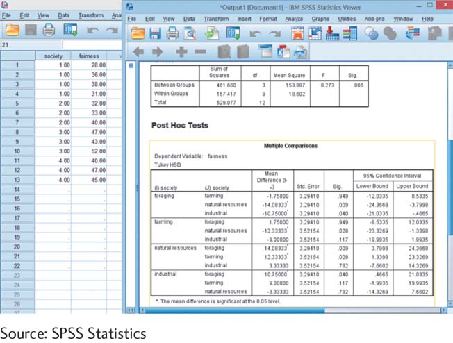
In this chapter we conducted a one-way between-groups ANOVA to compare people in four different types of societies in terms of how fairly they behaved in a game, as assessed by the proportion of money that they gave to a second player in that game. The type of society was a nominal independent variable, and the proportion of money that they gave to the second player was a scale dependent variable. To conduct a one-way between-groups ANOVA using SPSS, we enter the data so that each participant has one row with all of her or his data. For example, a person would have a score in the first column indicating the type of society, perhaps a 1 for foraging or a 3 for natural resources, and a score in the second column indicating fairness level, the proportion of money he or she gave to a second player. The data as they should be entered are visible behind the output on the screenshot shown here.
Then we can instruct SPSS to conduct the ANOVA by selecting Analyze → Compare Means → One-Way ANOVA. Now select the variables from the list. The independent variable, named “society” here, goes in the box marked “Factor,” and the dependent variable, named “fairness” here, goes in the box labeled “Dependent List.” To request a post hoc test to compare the means of the four groups, select “Post Hoc,” then “Tukey,” and then click “Continue.” Click “OK” to run the ANOVA.
On the screenshot, we can see the source table near the top. Notice that the sums of squares, degrees of freedom, mean squares, and F statistic match the ones we calculated earlier. Any slight differences are due to differences in rounding decisions. The last column, titled “Sig.,” says .006. This number indicates that the actual p value of this test statistic is just 0.006, which is less than the 0.05 p level typically used in hypothesis testing and an indication that we can reject the null hypothesis. Below the source table, we can see the output for the post hoc test. Mean differences with an asterisk are statistically significant at a p level of 0.05. The output here matches the post hoc test we conducted earlier.
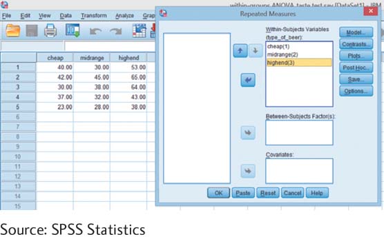
To conduct a one-way within-groups ANOVA on SPSS using the beer-rating data from the chapter, we enter the data so that each participant has one row with all of his data. This results in a different format from that of the data entered for a one-way between-groups ANOVA. In that case, we had a score for each participant’s level of the independent variable and a score for the dependent variable. For a within-groups ANOVA, each participant has multiple scores on the dependent variable. The levels of the independent variable are indicated in the titles for each of the three columns in SPSS. For example, as seen on the left of the SPSS screenshot, the first participant has scores of 40 for the cheap beer, 30 for the mid-range beer, and 53 for the high-end beer. Instruct SPSS to conduct the ANOVA by selecting Analyze → General Linear Model → Repeated Measures. (Remember that repeated measures is another way to say “within groups” when describing ANOVA.) Next, under “Within-Subject Factor Name,” change the generic “factor1” to the actual name of the independent variable, such as “type_of_beer” (using underscores between words because SPSS doesn’t recognize spaces in a variable name). Next to “Number of Levels,” type “3” to represent the number of levels of the independent variable in this study. Now click “Add,” followed by “Define.” Define the levels by clicking each of the three levels, then clicking the arrow button, in turn. You can see the entered data, and the box in which to define the levels, in the screenshot. To see the results of the ANOVA, click “OK.”
Page 311
The output includes more tables than in the between-groups ANOVA SPSS output. The one we want to pay attention to is titled “Tests of Within-Subjects Effects.” This table provides four F values and four “Sig.” values (the actual p values). There are several more advanced considerations that play into deciding which one to use; for the purposes of this introduction to SPSS, we simply note that the F values are all the same, and all match the F of 14.77 that we calculated previously. Moreover, all of the p values are less than the cutoff of 0.05. As we could when we conducted this one-way within-groups ANOVA by hand, we can reject the null hypothesis.