How It Works
11.1 CONDUCTING A ONE-
Irwin and colleagues (2004) are among a growing number of behavioral health researchers who are interested in adherence to medical regimens. These researchers studied adherence to an exercise regimen over one year in postmenopausal women, who are at increased risk for medical problems that may be reduced by exercise. Among the many factors that the research team examined was attendance at a monthly group education program that taught tactics to change exercise behavior; the researchers kept attendance and divided participants into three categories based on the number of sessions they attended. (Note: The researchers could have kept the data as numbers of sessions, a scale variable, rather than dividing them into categories based on numbers of sessions, an ordinal variable.)
Here is an abbreviated version of this study with fictional data points; the means of these data points, however, are the actual means of the study.
< 5 sessions: 155, 120, 130
5–
9–
In this study, the independent variable was attendance, with three levels: <5 sessions, 5–
Summary of Step 1
Population 1: Postmenopausal women who attended fewer than 5 sessions of a group exercise-
The comparison distribution will be an F distribution. The hypothesis test will be a one-
| Sample | < 5 | 5– |
9– |
| Squared deviations | 400 | 324 | 324 |
| 225 | 441 | 4 | |
| 25 | 9 | 289 | |
| 9 | |||
| Sum of squares | 650 | 774 | 626 |
| N – 1 | 2 | 2 | 3 |
| Variance | 325 | 387 | 208.67 |
Summary of Step 2
Null hypothesis: Postmenopausal women in different categories of attendance at a group exercise-
Summary of Step 3
dfbetween = Ngroups − 1 = 3 − 1 = 2
df1 = 3 − 1 = 2; df2 = 3 − 1 = 2; df3 = 4 − 1 = 3
dfwithin = 2 + 2 + 3 = 7
The comparison distribution will be the F distribution with 2 and 7 degrees of freedom.
Summary of Step 4
The critical F statistic based on a p level of 0.05 is 4.74.
Summary of Step 5
dftotal = 2 + 7 = 9 or dftotal = 10 − 1 = 9
SStotal = Σ(X − GM)2 = 12,222.40
| Sample | X | (X − GM) | (X − GM)2 | |
| < 5 | 155 | −24.6 | 605.16 | |
| M<5 = 135 | 120 | −59.6 | 3552.16 | |
| 130 | −49.6 | 2460.16 | ||
| 5– |
199 | 19.4 | 376.36 | |
| M5– |
160 | −19.6 | 384.16 | |
| 184 | 4.4 | 19.36 | ||
| 9– |
230 | 50.4 | 2540.16 | |
| M9– |
214 | 34.4 | 1183.36 | |
| 195 | 15.4 | 237.16 | ||
| 209 | 29.4 | 864.36 | ||
| GM = 179.60 | SStotal = 12,222.40 |
SSwithin = ∑ (X − M)2 = 2050.00
| Sample | X | (X − M) | (X − M)2 |
| < 5 | 155 | 20 | 400 |
| M<5 = 135 | 120 | −15 | 225 |
| 130 | −5 | 25 | |
| 5– |
199 | 18 | 324 |
| M5– |
160 | −21 | 441 |
| 184 | 3 | 9 | |
| 9– |
230 | 18 | 324 |
| M9– |
214 | 2 | 4 |
| 195 | −17 | 289 | |
| 209 | −3 | 9 | |
| GM = 179.60 | SSwithin = 2050.00 |
SSbetween = ∑(M − GM)2 = 10,172.40
| Sample | X | (M − GM) | (M − GM)2 |
| < 5 | 155 | −44.6 | 1989.16 |
| M<5 = 135 | 120 | −44.6 | 1989.16 |
| 130 | −44.6 | 1989.16 | |
| 5– |
199 | 1.4 | 1.96 |
| M5– |
160 | 1.4 | 1.96 |
| 184 | 1.4 | 1.96 | |
| 9– |
230 | 32.4 | 1049.76 |
| M9– |
214 | 32.4 | 1049.76 |
| 195 | 32.4 | 1049.76 | |
| 209 | 32.4 | 1049.76 | |
| GM = 179.60 | SSbetween = 10,172.40 |
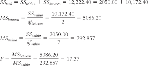
| Source | SS | df | MS | F |
| Between | 10,172.40 | 2 | 5,086.200 | 17.37 |
| Within | 2,050.00 | 7 | 292.857 | |
| Total | 12,222.40 | 9 |
Summary of Step 6
The F statistic, 17.37, is beyond the cutoff of 4.74. We can reject the null hypothesis. It appears that postmenopausal women in different categories of attendance at a group exercise-