Enter the data for the example used to calculate the correlation coefficient in this chapter: numbers of absences and exam grades. Be sure to put each student’s two scores on the same row.

To view a scatterplot, select: Graphs → Chart Builder → Gallery → Scatter/Dot. (Note: The first time you click “Chart Builder,” you may have to then click OK to indicate that you have correctly listed the variables as scale, ordinal, or nominal.) Drag the upper-left sample scatterplot to the large box on top. Then select the variables to be included in the scatterplot by dragging the independent variable, absences, to the x-axis and the dependent variable, grade, to the y-axis. Click “OK.”

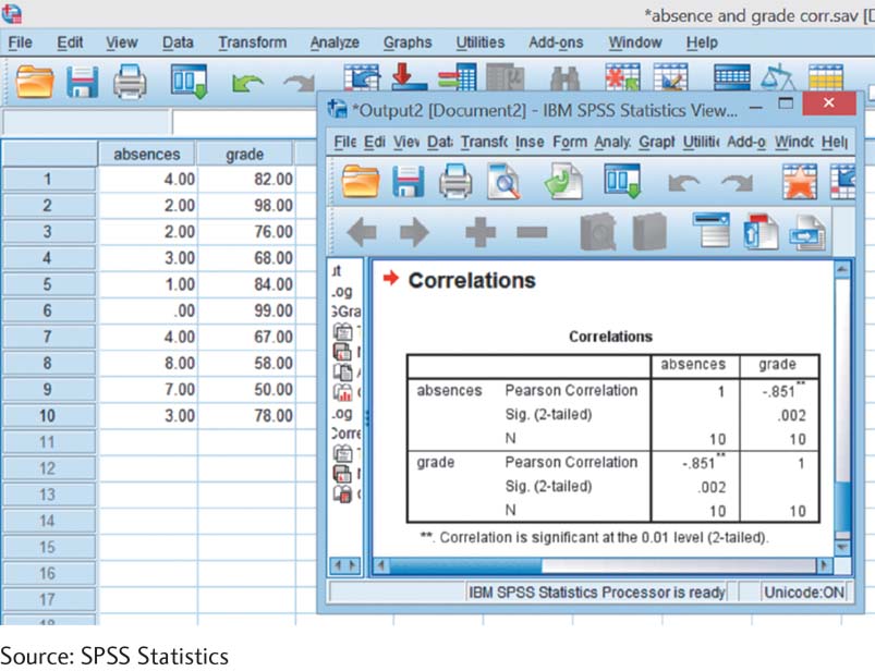
If the scatterplot indicates that we meet the assumptions for a Pearson correlation coefficient, we can analyze the data. Select: Analyze → Correlate → Bivariate. (Note: Bivariate means that you are analyzing two variables.) Then select the two variables to be analyzed, absences and grade. “Pearson” will already be checked as the type of correlation coefficient to be calculated. (Note: If more than two variables are selected, SPSS will build a correlation matrix of all possible pairs of variables.) Click “OK” to see the Output screen. The screenshot here shows the output for the Pearson correlation coefficient. Notice that the correlation coefficient is −0.851, the same as the coefficient that we calculated by hand earlier. The two asterisks indicate that it is statistically significant at a p level of less than 0.01. You can see under the correlation coefficient that the actual p value is 0.002.