14.1 REGRESSION WITH z SCORES

Shannon Callahan, a former student in the experimental psychology master’s program at Seton Hall University, conducted a study that examined evaluations of faculty members on Ratemyprofessor.com. She wondered if professors who were rated high on “clarity” were more likely to be viewed as “easy.” Callahan found a significant correlation of 0.267 between the average easiness rating a professor garnered and the average rating he or she received with respect to clarity of teaching.

419

If we know that a professor’s z score on clarity is 2.2 (an indication that she is very clear), how could we predict her z score on easiness?

z_Ŷ = (r_XY)(z_X) = (0.267)(2.2) = 0.59

When there’s a positive correlation, we predict a z score above the mean when her original z score is above the mean.

And if a professor’s z score on clarity is –1.8 (an indication that she’s not very clear), how could we predict her z score on easiness?

z_Ŷ = (r_XY)(z_X) = (0.267)(–1.8) = –0.48

When there’s a positive correlation, we predict a z score below the mean when her original z score is below the mean.

14.2 REGRESSION WITH RAW SCORES

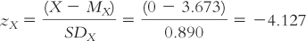
Using Shannon Callahan’s data, how can we develop the regression equation so that we can work directly with raw scores? To do this, we need a little more information. For this data set, the mean clarity score is 3.673, with a standard deviation of 0.890; the mean easiness score is 2.843, with a standard deviation of 0.701. As noted before, the correlation between these variables is 0.267.

To calculate the regression equation, we need to find the intercept and the slope. We determine the intercept by calculating what we predict for Y (easiness) when X (clarity) equals 0. Given the means, the standard deviations, and the correlation calculated above, we first find z_X:

We then calculate the predicted z score for easiness:

z_Ŷ = (r_XY)(z_X) = (0.267)(–4.127) = –1.102

Finally, we transform the predicted easiness z score into the predicted easiness raw score:

Ŷ = z_Ŷ (SD_Y) + M_Y = –1.102(0.701) + 2.843 = 2.070

The intercept, therefore, is 2.070.

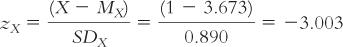
To determine the slope, we calculate what we would predict for Y (easiness) when X (clarity) equals 1, and determine how much that differs from what we would predict when X equals 0. The z score for X corresponding to the raw score of 1 is:

We then calculate the predicted z score for easiness:

z_Ŷ = (r_XY)(z_X) = (0.267)(–3.003) = –0.802

Finally, we transform the predicted easiness z score into the predicted easiness raw score:

Ŷ = z_Ŷ (SD_Y) + M_Y = –0.802(0.701) + 2.843 = 2.281

The difference between the predicted Y when X equals 1 (2.281) and that when X equals 0 (2.070) yields the slope, which is 2.281 – 2.070 = 0.211. So the regression equation is:

Ŷ = 2.07 + 0.21(X)

We can then use this regression equation to calculate a professor’s predicted easiness score from his or her clarity score. Let’s say a professor has a clarity score of 3.2. We would use the regression equation to predict her easiness score as follows:

Ŷ = 2.07 + 0.21(X) = 2.07 + 0.21(3.2) = 2.74

This result makes sense because she is below the mean on clarity, so, given that there is a positive correlation, we predict her score to fall below the mean on easiness.

420