15.2 Chi-
The chi-
square test for goodness of fit is a nonparametric hypothesis test that is used when there is one nominal variable.
The chi-
square test for independence is a nonparametric hypothesis test that is used when there are two nominal variables.
Hot-
433
MASTERING THE CONCEPT
15-
Both chi-
Chi-
The chi-
EXAMPLE 15.1
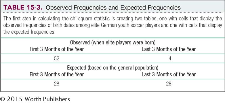
For example, researchers reported that the best youth soccer players in the world were more likely to have been born early in the year than later (Dubner & Levitt, 2006a). As one example, they reported that 52 elite youth players in Germany were born in January, February, or March, whereas only 4 players were born in October, November, or December. (Those born in other months were not included in this study.)
The null hypothesis predicts that when a person was born will not make any difference; the research hypothesis predicts that the month a person was born will matter when it comes to being an elite soccer player. Assuming that births in the general population are evenly distributed across months of the year, the null hypothesis posits that equal numbers of elite soccer players were born in the first 3 months and the last 3 months of the year. With 56 participants in the study (52 born in the first 3 months and 4 in the last 3 months), equal frequencies lead us to expect 28 players to have been born in the first 3 months and 28 in the last 3 months just by chance. The birth months don’t appear to be evenly distributed, but is this a real pattern, or just chance?

Like previous hypothesis tests, the chi-
STEP 1: Identify the populations, distribution, and assumptions.
There are always two populations involved in a chi-
434
The first assumption is that the variable (birth month) is nominal. The second assumption is that each observation is independent; no single participant can be in more than one category. The third assumption is that participants were randomly selected. If not, it may be unwise to confidently generalize beyond the sample. A fourth assumption is that there is a minimum number of expected participants in every category (also called a cell)—at least 5 and preferably more. An alternative guideline (Delucchi, 1983) is for there to be at least five times as many participants as cells. In any case, the chi-
Summary: Population 1: Elite German youth soccer players with birth dates like those we observed. Population 2: Elite German youth soccer players with birth dates like those in the general population.
The comparison distribution is a chi-
STEP 2: State the null and research hypotheses.
For chi-
Summary: Null hypothesis: Elite German youth soccer players have the same pattern of birth months as those in the general population. Research hypothesis: Elite German youth soccer players have a different pattern of birth months than those in the general population.
STEP 3: Determine the characteristics of the comparison distribution.
Our only task at this step is to determine the degrees of freedom. In most previous hypothesis tests, the degrees of freedom have been based on sample size. For the chi-
dfχ2 = k – 1
MASTERING THE FORMULA
15-
dfχ2 = k – 1
Here, k is the symbol for the number of categories. The current example has only two categories: Each soccer player in this study was born in either the first 3 months of the year or the last 3 months of the year:
dfχ2 = 2 – 1 = 1
Summary: The comparison distribution is a chi-
435
STEP 4: Determine the critical values, or cutoffs.
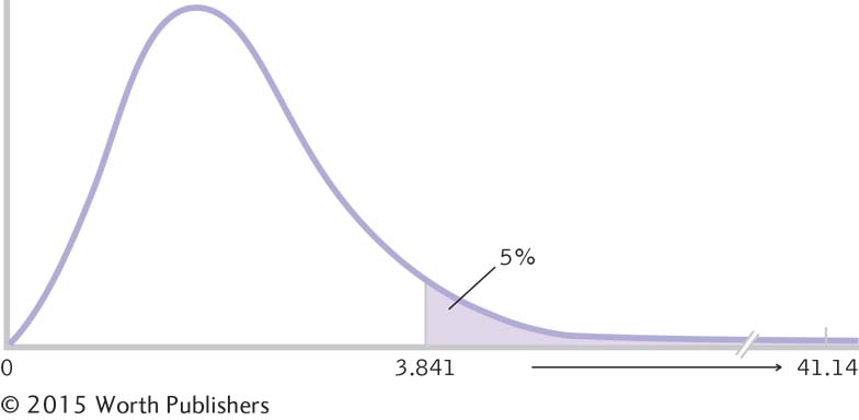
To determine the cutoff, or critical value, for the chi-
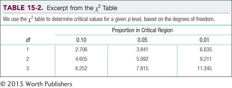
Summary: The critical χ2, based on a p level of 0.05 and 1 degree of freedom, is 3.841, as seen in the curve in Figure 15-1.
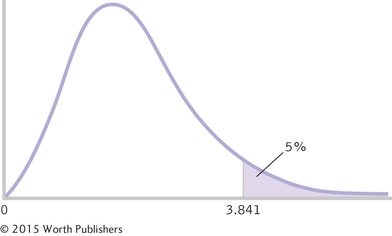
Determining the Cutoff for a Chi-
We look up the critical value for a chi-
STEP 5: Calculate the test statistic.
To calculate a chi-
(0.50)(56) = 28
Of the 56 elite German youth soccer players in the study, we would expect to find that 28 were born in the first 3 months of the year (versus the last 3 months of the year) if these youth soccer players are no different from the general population with respect to birth date. Similarly, we would expect a proportion of 1 − 0.50 = 0.50 of these soccer players to be born in the last 3 months of the year:
436
(0.50)(56) = 28
These numbers are identical only because the proportions are 0.50 and 0.50. If the proportion expected for the first 3 months of the year, based on the general population, were 0.60, then we would expect a proportion of 1 – 0.60 = 0.40 for the last 3 months of the year.
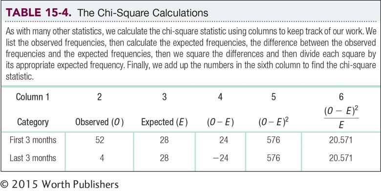
The next step in calculating the chi-
437
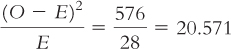
As an example, here are the calculations for the category “first 3 months”:
O − E = (52 − 28) = 24
(O − E)2 = (24)2 = 576
Once we complete the table, the last step is easy. We just add up the numbers in the sixth column. In this case, the chi-
Summary: 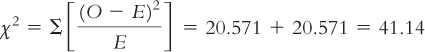
MASTERING THE FORMULA
15-
For each cell, we subtract the expected count, E, from the observed count, O. Then we square each difference and divide the square by the expected count. Finally, we sum the calculations for each of the cells.
STEP 6: Make a decision.
This last step is identical to that of previous hypothesis tests. We reject the null hypothesis if the test statistic is beyond the critical value, and we fail to reject the null hypothesis if the test statistic is not beyond the critical value. In this case, the test statistic, 41.14, is far beyond the cutoff, 3.841, as seen in Figure 15-2. We reject the null hypothesis. Because there are only two categories, it’s clear where the difference lies. It appears that elite German youth soccer players are more likely to have been born in the first 3 months of the year, and less likely to have been born in the last 3 months of the year, than members of the general population. (If we had failed to reject the null hypothesis, we could only have concluded that these data did not provide sufficient evidence to show that elite German youth soccer players have a different likelihood of being born in the first, versus last, 3 months of the year than those in the general population.)
Making a Decision
As with other hypothesis tests, we make a decision with a chi-

Summary: Reject the null hypothesis; it appears that elite German youth soccer players are more likely to have been born in the first 3 months of the year, and less likely to have been born in the last 3 months of the year, than people in the general population.
438
We report these statistics in a journal article in almost the same format that we’ve seen previously. We report the degrees of freedom, the value of the test statistic, and whether the p value associated with the test statistic is less than or greater than the cutoff based on the p level of 0.05. (As usual, we would report the actual p level if we conducted this hypothesis test using software.) In addition, we report the sample size in parentheses with the degrees of freedom. In the current example, the statistics read:
χ2(1, N = 56) = 41.14, p < 0.05
The researchers who conducted this study imagined four possible explanations: “a) certain astrological signs confer superior soccer skills; b) winter-
Dubner and Levitt (2006a) picked (d) and suggested another alternative. Participation in youth soccer leagues has a strict cutoff date: December 31. Compared to those born in December, children born the previous January are likely to be more physically and emotionally mature, perceived as more talented, chosen for the best leagues, and given better coaching—
Chi-
The chi-
Like the correlation coefficient, the chi-
EXAMPLE 15.2
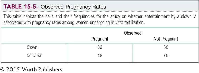
In the clown study, as reported in the mass media (Ryan, 2006), 186 women were randomly assigned to receive IVF treatment only or to receive IVF treatment followed by 15 minutes of clown entertainment. Eighteen of the 93 who received only the IVF treatment became pregnant, whereas 33 of the 93 who received both IVF treatment and clown entertainment became pregnant. The cells for these observed frequencies can be seen in Table 15-5. The table of cells for a chi-
439
STEP 1: Identify the populations, distribution, and assumptions.
Population 1: Women receiving IVF treatment like the women we observed. Population 2: Women receiving IVF treatment for whom the presence of a clown is not associated with eventual pregnancy.
The comparison distribution is a chi-
STEP 2: State the null and research hypotheses.
Null hypothesis: Pregnancy rates are independent of whether one is entertained by a clown after IVF treatment. Research hypothesis: Pregnancy rates depend on whether one is entertained by a clown after IVF treatment.
STEP 3: Determine the characteristics of the comparison distribution.
For a chi-
dfrow = krow − 1
MASTERING THE FORMULA
15-
The degrees of freedom for the variable in the columns of the contingency table are:
dfcolumn = kcolumn − 1
The overall degrees of freedom are:
dfχ2 = (dfrow)(dfcolumn)
To expand this last formula, we write:
dfχ2 = (krow – 1)(kcolumn – 1)
The comparison distribution is a chi-
dfχ2 = (krow – 1)(kcolumn – 1) = (2 – 1)(2 – 1) = 1
440
STEP 4: Determine the critical value, or cutoff.
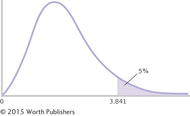
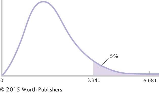
The critical value, or cutoff, for the chi-
The Cutoff for a Chi-
The shaded region is beyond the critical value for a chi-
STEP 5: Calculate the test statistic.
The next step, determining the appropriate expected frequencies, is the most important in the calculation of the chi-
But this would not make sense. Of the 186 women, only 51 became pregnant; 51/186 = 0.274, or 27.4%, of these women became pregnant. If pregnancy rates do not depend on clown entertainment, then we would expect the same percentage of successful pregnancies, 27.4%, regardless of exposure to clowns. If we have expected frequencies of 46.5 in all four cells, then we have a 50%, not a 27.4%, pregnancy rate. We must always consider the specifics of the situation.
In the current study, we already calculated that 27.4% of all women in the study became pregnant. If pregnancy rates are independent of whether a woman is entertained by a clown, then we would expect 27.4% of the women who were entertained by a clown to become pregnant and 27.4% of women who were not entertained by a clown to become pregnant. Based on this percentage, 100 − 27.4 = 72.6% of women in the study did not become pregnant. We would therefore expect 72.6% of women who were entertained by a clown to fail to become pregnant and 72.6% of women who were not entertained by a clown to fail to become pregnant. Again, we expect the same pregnancy and nonpregnancy rates in both groups—
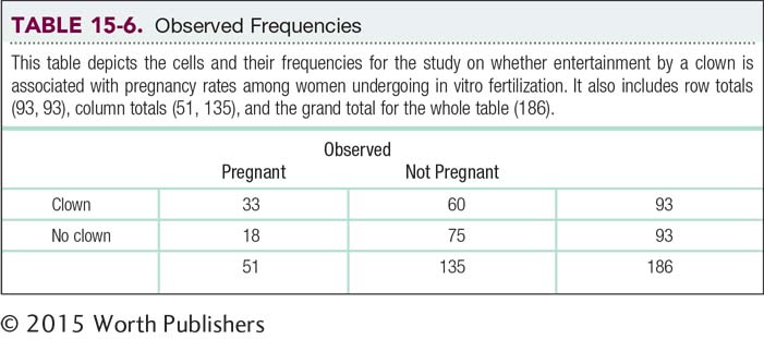
Table 15-6 shows the observed data, and it also shows totals for each row, each column, and the whole table. From Table 15-6, we see that 93 women were entertained by a clown after IVF treatment. As we calculated above, we would expect 27.4% of them to become pregnant:
(0.274)(93) = 25.482
Of the 93 women who were not entertained by a clown, we would expect 27.4% to become pregnant if clown entertainment is independent of pregnancy rates:
(0.274)(93) = 25.482
441
We now repeat the same procedure for not becoming pregnant. We would expect 72.6% of women in both groups to not become pregnant. For the women who were entertained by a clown, we would expect 72.6% of them to not become pregnant:
(0.726)(93) = 67.518
Of the women who were not entertained by a clown, we would expect 72.6% to not become pregnant:
(0.726)(93) = 67.518
(Note that the two expected frequencies for the first row are the same as the two expected frequencies for the second row, but only because the same number of people were in each clown condition, 93. If these two numbers were different, we would not see the same expected frequencies in the two rows.)
MASTERING THE FORMULA
15-
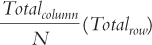
The method of calculating the expected frequencies that we described above is ideal because it is directly based on our own thinking about the frequencies in the rows and in the columns. Sometimes, however, our thinking can get muddled, particularly when the two (or more) row totals do not match and the two (or more) column totals do not match. For these situations, a simple set of rules leads to accurate expected frequencies. For each cell, we divide its column total (Totalcolumn) by the grand total (N) and multiply that by the row total (Totalrow):
As an example, the observed frequency of those who became pregnant and were entertained by a clown is 33. The row total for this cell is 93. The column total is 51. The grand total, N, is 186. The expected frequency, therefore, is:

Notice that this result is identical to what we calculated without a formula. The middle step above shows that, even with the formula, we actually did calculate the pregnancy rate overall, by dividing the column total (51) by the grand total (186). We then calculated how many in that row of 93 participants we would expect to become pregnant using this overall rate:
(0.274)(93) = 25.482
442
The formula follows the logic of the test, and keeps us on track when there are multiple calculations.
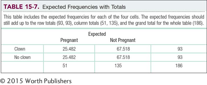
As a final check on the calculations, shown in Table 15-7, we can add up the frequencies to be sure that they still match the row, column, and grand totals. For example, if we add the two numbers in the first column, 25.482 and 25.482, we get 50.964 (different from 51 only because of rounding decisions). If we had made the mistake of dividing the 186 participants into cells by dividing by 4, we would have had 46.5 in each cell; then the total for the first column would have been 46.5 + 46.5 = 93, which is not a match with 51. This final check ensures that we have the appropriate expected frequencies in the cells.
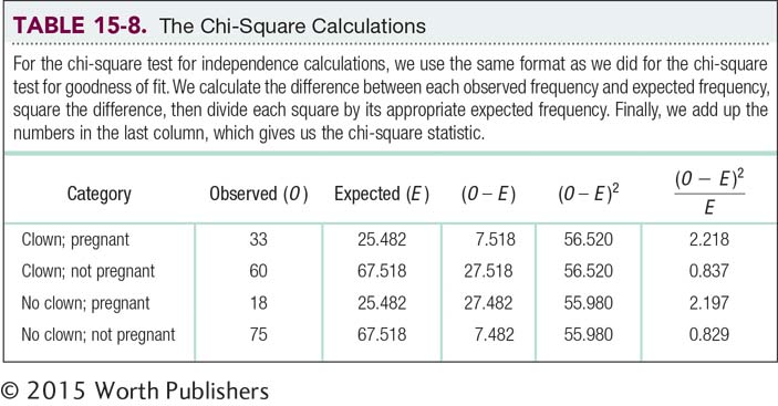
The remainder of the fifth step is identical to that for a chi-

STEP 6: Make a decision.
Reject the null hypothesis; it appears that pregnancy rates depend on whether a woman receives clown entertainment following IVF treatment (Figure 15-4). The statistics, as reported in a journal article, would follow the format we learned for a chi-
χ2(1, N = 186) = 6.08, p < 0.05
The Decision
Because the chi-
443
Cramér’s V, the Effect Size for Chi Square
A hypothesis test tells us only that there is a likely effect—
MASTERING THE FORMULA
15-
Cramér’s 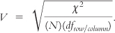
The numerator is the chi-
Cramér’s V is the standard effect size used with the chi-
square test for independence; also called Cramér’s phi, symbolized as
Cramér’s V is the standard effect size used with the chi-
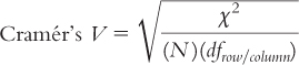
χ2 is the test statistic we just calculated, N is the total number of participants in the study (the lower-
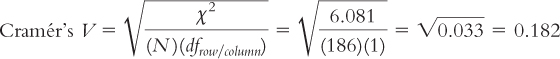
EXAMPLE 15.3
For the clown example, we calculated a chi-
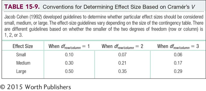
Now that we have the effect size, we must ask what it means. As with other effect sizes, Jacob Cohen (1992) has developed guidelines, shown in Table 15-9, for determining whether a particular effect is small, medium, or large. The guidelines vary based on the size of the contingency table. When the smaller of the two degrees of freedom for the row and column is 1, we use the guidelines in the second column. When the smaller of the two degrees of freedom is 2, we use the guidelines in the third column. And when it is 3, we use the guidelines in the fourth column. As with the other guidelines for judging effect sizes, such as those for Cohen’s d, the guidelines are not cutoffs. Rather, they are rough indicators to help researchers gauge a finding’s importance.
444
The effect size for the clowning and pregnancy study was 0.18. The smaller of the two degrees of freedom, that for the row and that for the column, was 1 (in fact, both were 1). So we use the second column in Table 15-9. This Cramér’s V falls about halfway between the effect-
χ2(1, N = 186) = 6.08, p < Cramér’s V = 0.18
Graphing Chi-
In addition to calculating Cramér’s V, we can graph the data. A visual depiction of the pattern of results is an effective way to understand the size of the relation between two variables assessed using the chi-
EXAMPLE 15.4
For the women entertained by a clown, we calculate the proportion who became pregnant and the proportion who did not. For the women not entertained by a clown, we again calculate the proportion who became pregnant and the proportion who did not. The calculations for the proportions are below.
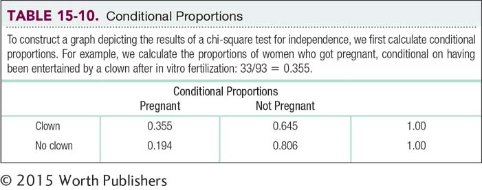
In each case, we’re dividing the number of a given outcome by the total number of women in that group. The proportions are called conditional proportions because we’re not calculating the proportions out of all women in the study; we’re calculating proportions for women in a certain condition. We calculate the proportion of women who became pregnant, for example, conditional on their having been entertained by a clown.
Entertained by a clown
Became pregnant: 33/93 = 0.355
Did not become pregnant: 60/93 = 0.645
Not entertained by a clown
Became pregnant: 18/93 = 0.194
Did not become pregnant: 75/93 = 0.806
445
We can put those proportions into a table (such as Table 15-10). For each category of entertainment (clown, no clown), the proportions should add up to 1.00; or if we used percentages, they should add up to 100%.
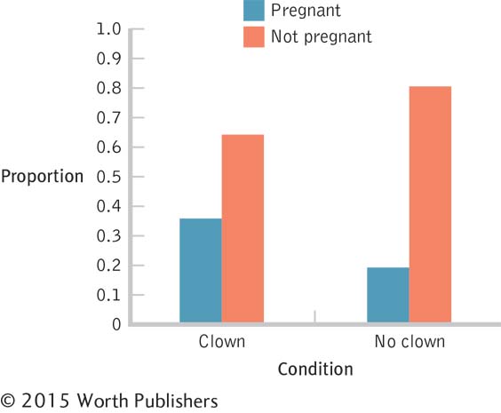
We can now graph the conditional proportions, as in Figure 15-5. Alternately, we could have simply graphed the two rates at which women got pregnant—
Graphing and Chi Square
When we graph the data for a chi-
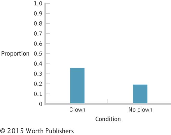
A Simpler Graph of Conditional Probabilities
Because the rates at which women did not become pregnant are based on the rates at which they did become pregnant, we can simply graph one set of rates. Here we see the rates at which women became pregnant in each of the two clown conditions.
Relative Risk
Relative risk is a measure created by making a ratio of two conditional proportions; also called relative likelihood or relative chance.
Public health statisticians like John Snow (Chapter 1) are called epidemiologists. They often think about the size of an effect with chi square in terms of relative risk, a measure created by making a ratio of two conditional proportions. It is also called relative likelihood or relative chance.
446
EXAMPLE 15.5
As with Figure 15-5, we calculate the chance of getting pregnant with clown entertainment after IVF by dividing the number of pregnancies in this group by the total number of women entertained by clowns:
33/93 = 0.355
MASTERING THE CONCEPT
15-
We then calculate the chance of getting pregnant with no clown entertainment after IVF by dividing the number of pregnancies in this group by the total number of women not entertained by clowns:
18/93 = 0.194
If we divide the chance of getting pregnant having been entertained by clowns by the chance of getting pregnant not having been entertained by clowns, then we get the relative likelihood:
0.355/0.194 = 1.830
Based on the relative risk calculation, the chance of getting pregnant when IVF is followed by clown entertainment is 1.83 times (or about twice) the chance of getting pregnant when IVF is not followed by clown entertainment. This matches the impression that we get from the graph.
Alternately, we can reverse the ratio, dividing the chance of becoming pregnant without clown entertainment, 0.194, by the chance of becoming pregnant following clown entertainment, 0.355. This is the relative likelihood for the reversed ratio:
0.194/0.355 = 0.546
This number gives us the same information in a different way. The chance of getting pregnant when IVF is followed by no entertainment is 0.55 (or about half) the chance of getting pregnant when IVF is followed by clown entertainment. Again, this matches the graph; one bar is about half that of the other.

(Note: When this calculation is made with respect to diseases, it is referred to as relative risk [rather than relative likelihood].) We should be careful when relative risks and relative likelihoods are reported, however. We must always be aware of base rates. If, for example, a certain disease occurs in just 0.01% of the population (that is, 1 in 10,000) and is twice as likely to occur among people who eat ice cream, then the rate is 0.02% (2 in 10,000) among those who eat ice cream. Relative risks and relative likelihoods can be used to scare the general public unnecessarily—
447
CHECK YOUR LEARNING
| Reviewing the Concepts |
|
|
| Clarifying the Concepts | 15- |
When do we use chi- |
| 15- |
What are observed frequencies and expected frequencies? | |
| 15- |
What is the effect- |
|
| Calculating the Statistics | 15- |
Imagine a town that boasts clear blue skies 80% of the time. You get to work in that town one summer for 78 days and record the following data. (Note: For each day, you picked just one label.) Clear blue skies: 59 days Cloudy/hazy/gray skies: 19 days 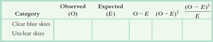
|
| 15- |
Assume you are interested in whether students with different majors tend to have different political affiliations. You ask U.S. psychology majors and business majors to indicate whether they are Democrats or Republicans. Of 67 psychology majors, 36 indicated that they are Republicans and 31 indicated that they are Democrats. Of 92 business majors, 54 indicated that they are Republicans and 38 indicated that they are Democrats. Calculate the relative likelihood of being a Republican, given that a person is a business major as opposed to a psychology major. | |
| Applying the Concepts | 15- |
The Chicago Police Department conducted a study comparing two types of lineups for suspect identification: simultaneous lineups and sequential lineups (Mecklenburg, Malpass, & Ebbesen, 2006). In simultaneous lineups, witnesses saw the suspects all at once, either live or in photographs, and then made their selection. In sequential lineups, witnesses saw the people in the lineup one at a time, either live or in photographs, and said yes or no to suspects one at a time. After numerous high-
|
Solutions to these Check Your Learning questions can be found in Appendix D.