Exercises
Clarifying the Concepts
Question 15.1
| 15.1 |
Distinguish among nominal, ordinal, and scale data. |
Question 15.2
| 15.2 |
What are the three main situations in which we use a nonparametric test? |
Question 15.3
| 15.3 |
What is the difference between the chi- |
Question 15.4
| 15.4 |
What are the four assumptions for the chi- |
Question 15.5
| 15.5 |
List two ways in which statisticians use the word independence or independent with respect to concepts introduced earlier in this book. Then describe how independence is used by statisticians with respect to chi square. |
Question 15.6
| 15.6 |
What are the hypotheses when conducting the chi- |
Question 15.7
| 15.7 |
How are the degrees of freedom for the chi- |
Question 15.8
| 15.8 |
Why is there just one critical value for a chi- |
Question 15.9
| 15.9 |
What information is presented in a contingency table in the chi- |
Question 15.10
| 15.10 |
What measure of effect size is used with chi square? |
Question 15.11
| 15.11 |
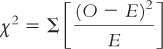
Define the symbols in the following formula: |
Question 15.12
| 15.12 |
What is the formula |
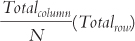 used for?
Question 15.13
| 15.13 |
What information does the measure of relative likelihood provide? |
Question 15.14
| 15.14 |
In order to calculate relative likelihood, what must we first calculate? |
Question 15.15
| 15.15 |
What is the difference between relative likelihood and relative risk? |
Question 15.16
| 15.16 |
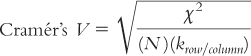
Why might relative likelihood be easier to understand as an effect size than Cramér’s V ? |
Question 15.17
| 15.17 |
Which graph is most useful for displaying the results of a chi- |
Question 15.18
| 15.18 |
Why can relative likelihood and relative risk sometimes exaggerate risks? (Hint: Think about the base rates— |
Question 15.19
| 15.19 |
When do we convert scale data to ordinal data? |
Question 15.20
| 15.20 |
When the data on at least one variable are ordinal, the data on any scale variable must be converted from scale to ordinal. How do we convert a scale variable into an ordinal one? |
Question 15.21
| 15.21 |
How does the transformation of scale data to ordinal data solve the problem of outliers? |
Question 15.22
| 15.22 |
What does a histogram of rank- |
Question 15.23
| 15.23 |
Explain how the relation between ranks is the core of the Spearman rank- |
Question 15.24
| 15.24 |
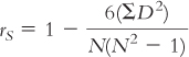
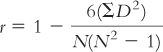
Define the symbols in the following term: |
Question 15.25
| 15.25 |
What is the possible range of values for the Spearman rank- |
Question 15.26
| 15.26 |
How would you respond in a situation in which you are ranking a set of scale data and there are two numbers that are exactly the same? |
Question 15.27
| 15.27 |
When is it appropriate to use the Wilcoxon signed- |
Question 15.28
| 15.28 |
When do we use the Mann– |
Question 15.29
| 15.29 |
What are the assumptions of the Mann– |
Question 15.30
| 15.30 |
How are the critical values for the Mann– |
Question 15.31
| 15.31 |
If the data meet the assumptions of the parametric test, why is it preferable to use the parametric test rather than the nonparametric alternative? |
Calculating the Statistics
Question 15.32
| 15.32 |
For each of the following, (i) identify the incorrect symbol, (ii) state what the correct symbol should be, and (iii) explain why the initial symbol was incorrect.
|

Question 15.33
| 15.33 |
For each of the following, identify the independent variable(s), the dependent variable(s), and the level of measurement (nominal, ordinal, scale).
|
Question 15.34
| 15.34 |
Use this calculation table for the chi-
|

Question 15.35
| 15.35 |
Use this calculation table for the chi-
|
Question 15.36
| 15.36 |
Below are some data to use in a chi-
|
||||||||||||||||||||||||||||||||
Question 15.37
| 15.37 |
The data below are from a study of lung cancer patients in Turkey (Yilmaz et al., 2000). Use these data to calculate the relative likelihood of the patient being a smoker, given that a person is female rather than male.
|
Question 15.38
| 15.38 |
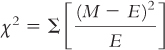
In order to compute statistics, we need to have working formulas. For the following, (i) identify the incorrect symbol, (ii) state what the correct symbol should be, and (iii) explain why the initial symbol was incorrect. |
Question 15.39
| 15.39 |
Consider the following scale data.
|
Question 15.40
| 15.40 |
Consider the following scale data.
|
Question 15.41
| 15.41 |
The following fictional data represent the finishing place for runners of a 5-
|
Question 15.42
| 15.42 |
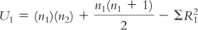
Compute the Mann–
|
Question 15.43
| 15.43 |
Compute the Mann–
|
Question 15.44
| 15.44 |
Assume a researcher compared the performance of two independent groups of participants on an ordinal variable using the Mann–
|
Question 15.45
| 15.45 |
Are men or women more likely to be at the top of their class? The following table depicts fictional class standings for a group of men and women:
|
Applying the Concepts
Question 15.46
| 15.46 |
A nonparametric test and gender differences in obeying bicycling laws: Students at Hunter College studied bicycle safety in New York City (Tuckel & Milczarski, 2014). They reported data on cyclists who were riding their own bikes and were not cycling as part of their job (they were not, for example, riding as delivery workers). They reported that 28.4% of male cyclists stopped completely at a red light, whereas 38.3% of female cyclists did so. 30.9% of male cyclists and 35.4% of female cyclists paused but then rolled through the red light. And 40.7% of male cyclists and 26.3% of female cyclists just ran the light. What hypothesis test would the researchers conduct? Explain your answer. |
Question 15.47
| 15.47 |
Gender, salary negotiation, and chi square: Researchers investigated whether or not language in job postings affected the likelihood that women and men would negotiate regarding salary (Leibbrandt & List, 2012). Some job postings clearly indicated that the salary was negotiable, and others contained no such statement. The postings were otherwise identical. The researchers examined the behavior of almost 2500 applicants for one of the jobs in these advertisements. The graph shows the proportions of women and men who negotiated in response to either type of listing. 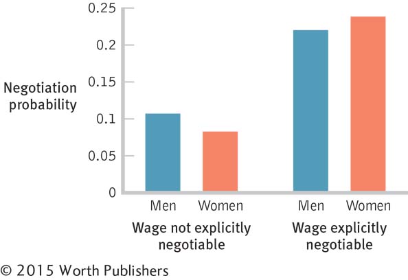
|
Question 15.48
| 15.48 |
Gender, the Oscars, and nonparametric tests: In 2010, Sandra Bullock won an Academy Award for best actress. Shortly thereafter, she discovered that her husband was cheating on her. Headlines erupted about a supposed Oscar curse that befalls women, and many in the media wondered whether ambitious women—
|
Question 15.49
| 15.49 |
Parametric or nonparametric test? For each of the following research questions, state whether a parametric or nonparametric hypothesis test is more appropriate. Explain your answers.
|
Question 15.50
| 15.50 |
Types of variables and student evaluations of professors: Weinberg, Fleisher, and Hashimoto (2007) studied almost 50,000 students’ evaluations of their professors in nearly 400 economics courses at the Ohio State University over a 10- I— II— III— Explain your answer to part (iii).
|
Question 15.51
| 15.51 |
Grade inflation and types of variables: A New York Times article on grade inflation reported several findings related to a tendency for average grades to rise over the years and a tendency for the top- I— II— III— Explain your answer to part (iii).
|
Question 15.52
| 15.52 |
High school academic performance and types of variables: Here are three ways to assess one’s performance in high school: (1) GPA at graduation, (2) whether one graduated with honors (as indicated by graduating with a GPA of at least 3.5), and (3) class rank at graduation. For example, Abdul had a 3.98 GPA, graduated with honors, and was ranked 10th in his class.
|
Question 15.53
| 15.53 |
Immigration, crime, and research design: “Do Immigrants Make Us Safer?” asked the title of a New York Times Magazine article (Press, 2006). The article reported findings from several U.S.-based studies, including several conducted by Harvard sociologist Robert Sampson in Chicago. For each of the following findings, draw the table of cells that would comprise the research design. Include the labels for each row and column.
|
Question 15.54
| 15.54 |
Sex selection and hypothesis testing: Across all of India, there are only 933 girls for every 1000 boys (Lloyd, 2006), evidence of a bias that leads many parents to illegally select for boys or to kill their infant girls. (Note that this translates into a proportion of girls of 0.483.) In Punjab, a region of India in which residents tend to be more educated than in other regions, there are only 798 girls for every 1000 boys. Assume that you are a researcher interested in whether sex selection is more or less prevalent in educated regions of India, and that 1798 children from Punjab constitute the entire sample. (Hint: You will use the proportions from the national database for comparison.)
|
Question 15.55
| 15.55 |
Gender, op-
|
Question 15.56
| 15.56 |
Romantic music, behavior, chi square, and effect size: Guéguen, Jacob, and Lamy (2010) investigated whether exposure to romantic music affects dating behavior. The participants, young, single French women, waited for the experiment to start in a room in which songs with either romantic lyrics or neutral lyrics were playing. After a few minutes, each woman who participated completed a marketing survey administered by a young male confederate. During a break, the confederate asked the participant for her phone number. Of the women who listened to romantic music, 52.2% (23 out of 44) gave him her phone number, whereas 27.9% (12 out of 43) of the women who listened to neutral music did so. The researchers conducted a chi-
|
Question 15.57
| 15.57 |
The General Social Survey, an exciting life, and relative risk: In How It Works 15.2, we walked through a chi-
|
Question 15.58
| 15.58 |
Page 472
Gender, ESPN, and chi square: Many of the numbers we see in the news could be analyzed with chi square. The feminist blog Culturally Disoriented examined the photos in the 2012 “body issue” of ESPN The Magazine—the publication’s annual spread of photographs of nude athletes. The blogger reported: “Female athlete after female athlete was photographed not as a talented, powerful sportswoman, but as. . .eye candy” (http:/
|
Question 15.59
| 15.59 |
Premarital doubts, divorce, and chi square: In an article titled “Do Cold Feet Warn of Trouble Ahead?”, researchers studied 464 married heterosexual spouses to determine whether or not doubts before marriage were predictive of marital troubles, and divorce, later on (Lavner, Karney, & Bradbury, 2012). The following is an excerpt from the results section of their paper: “For husbands, 9% of those who reported not having premarital doubts divorced by four years (n = 10 of 117) compared with 14% of those who did report premarital doubts (n = 15 of 106); these groups did not differ significantly, χ2 (1, n = 223) = 1.76, p > .10. Among wives, 8% of those who reported not having premarital doubts divorced by four years (n = 11 of 141) compared with 19% of those who did report premarital doubts (n = 16 of 84). Chi-
|
Question 15.60
| 15.60 |
University students, cell phone bills, and ordinal data: Here are some monthly cell phone bills, in dollars, for university students:
|
Question 15.61
| 15.61 |
World cities, livability, and nonparametric hypothesis tests: CNN.com reported on a 2012 study that ranked the world’s cities in terms of how livable they are (http:/
|
Question 15.62
| 15.62 |
Fantasy baseball and the Spearman correlation coefficient: In fantasy baseball, groups of 12 league participants conduct a draft in which they can “buy” any baseball players from any teams across one of the two Major League Baseball (MLB) leagues (the American League and the National League). These makeshift teams are compared on the basis of the combined statistics of the individual baseball players. For example, statistics about home runs are transformed into points, and each fantasy team receives a total score of all combined points based on its baseball players, regardless of their real-
|
Question 15.63
| 15.63 |
Test-
1.00, −0.001, 0.52, −0.27, −0.98, 0.09 Specify which of these coefficients suggests the strongest relation between the two variables as well as which coefficient suggests the weakest relation between the two variables. |
Question 15.64
| 15.64 |
Nonparametric tests and a longitudinal study of mathematically gifted teenagers: Researchers studied male and female teenagers who had scored in the top 1% on mathematical reasoning measures (Lubinski, Benbow, & Kell, 2014). The researchers were able to follow the participants’ progression over the next 40 years. They tracked two groups, or cohorts, of participants on a number of variables, including career- Page 474
|
Question 15.65
| 15.65 |
Public versus private universities and the Mann–
|
Question 15.66
| 15.66 |
Gender, aggression, and the interpretation of a Mann–
|
Question 15.67
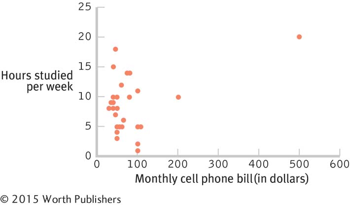
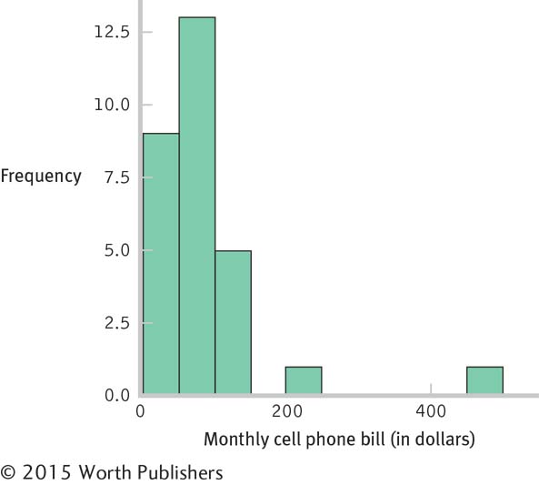
| 15.67 |
Cell phone bill, hours spent studying, and the shapes of distributions: The following figures display data that depict the relation between students’ monthly cell phone bills and the number of hours they report that they study per week.
|
Putting It All Together
Question 15.68
| 15.68 |
Stroke patients, treatment, and type of nonparametric test: A common situation faced by researchers working with special populations, such as neurologically impaired people or people with less common psychiatric conditions, is that the studies often have small sample sizes due to the relatively few number of patients. As a result, these researchers often turn to nonparametric statistical tests. For each of the following research descriptions, state which nonparametric hypothesis test is most appropriate: the Spearman rank-
|
Question 15.69
| 15.69 |
Gender bias, poor growth, and hypothesis testing: Grimberg, Kutikov, and Cucchiara (2005) wondered whether gender biases were evident in referrals of children for poor growth. They believed that boys were more likely to be referred even when there was no problem— Page 476
|
Question 15.70
| 15.70 |
The prisoner’s dilemma, cross-
|